Spectral analysis of a two frequencies signal

Context

Example

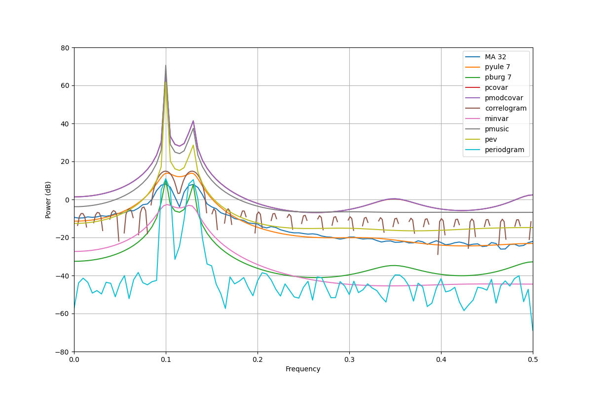
In the following example, we use most of the methods available to analyse an input signal made of the addition of two sinus and an additive gaussian noise

import numpy
import spectrum
from spectrum import tools
from numpy.testing import assert_array_almost_equal
import pylab
data = spectrum.marple_data

from pylab import *
nn = numpy.arange(200)
xx = cos(0.257*pi*nn) + sin(0.2*pi*nn) + 0.01*randn(size(nn));

def create_all_psd():

    f = pylab.linspace(0, 1, 4096)

    pylab.figure(figsize=(12,8))

    # MA model
    p = spectrum.pma(xx, 64,128); p(); p.plot()
    """
    #ARMA 15 order
    a, b, rho = spectrum.arma_estimate(data, 15,15, 30)
    psd = spectrum.arma2psd(A=a,B=b, rho=rho)
    newpsd = tools.cshift(psd, len(psd)//2) # switch positive and negative freq
    pylab.plot(f, 10 * pylab.log10(newpsd/max(newpsd)), label='ARMA 15,15')
    """
    # YULE WALKER
    p = spectrum.pyule(xx, 7 , NFFT=4096, scale_by_freq=False); p.plot()
    # equivalent to
    # plot([x for x in p.frequencies()] , 10*log10(p.psd)); grid(True)

    #burg method
    p = spectrum.pburg(xx, 7, scale_by_freq=False);  p.plot()

    #pcovar
    p = spectrum.pcovar(xx, 7, scale_by_freq=False);  p.plot()

    #pmodcovar
    p = spectrum.pmodcovar(xx, 7, scale_by_freq=False); p.plot()

    # correlogram
    p = spectrum.pcorrelogram(xx, lag=60, NFFT=512, scale_by_freq=False); p.plot()

    # minvar
    p = spectrum.pminvar(xx, 7, NFFT=256, scale_by_freq=False); p.plot()

    # pmusic
    p = spectrum.pmusic(xx, 10,4, scale_by_freq=False); p.plot()

    # pmusic
    p = spectrum.pev(xx, 10, 4, scale_by_freq=False); p.plot()

    # periodogram
    p = spectrum.Periodogram(xx, scale_by_freq=False); p.plot()

    #
    legend( ["MA 32", "pyule 7", "pburg 7", "pcovar", "pmodcovar", "correlogram",
                "minvar", "pmusic", "pev", "periodgram"])


    pylab.ylim([-80,80])

create_all_psd()

Total running time of the script: (0 minutes 0.326 seconds)

Download Python source code: plot_allpsd.py

Download IPython notebook: plot_allpsd.ipynb