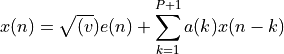
5.3. Parametric methods
5.3.1. Power Spectrum Density based on Parametric Methods
5.3.1.1. ARMA and MA estimates (yule-walker)
ARMA and MA estimates, ARMA and MA PSD estimates.
- arma2psd(A=None, B=None, rho=1.0, T=1.0, NFFT=4096, sides='default', norm=False)[source]
Computes power spectral density given ARMA values.
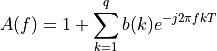
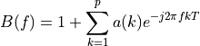
This function computes the power spectral density values given the ARMA parameters of an ARMA model. It assumes that the driving sequence is a white noise process of zero mean and variance
 . The sampling frequency and noise variance are
used to scale the PSD output, which length is set by the user with the
NFFT parameter.
. The sampling frequency and noise variance are
used to scale the PSD output, which length is set by the user with the
NFFT parameter.- Parameters:
A (array) – Array of AR parameters (complex or real)
B (array) – Array of MA parameters (complex or real)
rho (float) – White noise variance to scale the returned PSD
T (float) – Sampling frequency in Hertz to scale the PSD.
NFFT (int) – Final size of the PSD
sides (str) – Default PSD is two-sided, but sides can be set to centerdc.
Warning
By convention, the AR or MA arrays does not contain the A0=1 value.
If
Bis None, the model is a pure AR model. IfAis None, the model is a pure MA model.- Returns:
two-sided PSD
Details:
AR case: the power spectral density is:
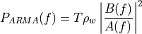
where:
Example:
import spectrum.arma
from pylab import plot, log10, legend
plot(10*log10(spectrum.arma.arma2psd([1,0.5],[0.5,0.5])), label='ARMA(2,2)')
plot(10*log10(spectrum.arma.arma2psd([1,0.5],None)), label='AR(2)')
plot(10*log10(spectrum.arma.arma2psd(None,[0.5,0.5])), label='MA(2)')
legend()
(
Source code,png,hires.png,pdf)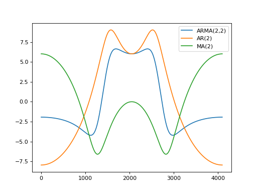
- References:
- arma_estimate(X, P, Q, lag)[source]
Autoregressive and moving average estimators.
This function provides an estimate of the autoregressive parameters, the moving average parameters, and the driving white noise variance of an ARMA(P,Q) for a complex or real data sequence.
The parameters are estimated using three steps:
Estimate the AR parameters from the original data based on a least squares modified Yule-Walker technique,
Produce a residual time sequence by filtering the original data with a filter based on the AR parameters,
Estimate the MA parameters from the residual time sequence.
- Parameters:
- Returns:
A - Array of complex P AR parameter estimates
B - Array of complex Q MA parameter estimates
RHO - White noise variance estimate
Note
lag must be >= Q (MA order)
from spectrum import arma_estimate, arma2psd, marple_data
import pylab

a,b, rho = arma_estimate(marple_data, 15, 15, 30)
psd = arma2psd(A=a, B=b, rho=rho, sides='centerdc', norm=True)
pylab.plot(10 * pylab.log10(psd))
pylab.ylim([-50,0])
(
Source code,png,hires.png,pdf)
- Reference:
- ma(X, Q, M)[source]
Moving average estimator.
This program provides an estimate of the moving average parameters and driving noise variance for a data sequence based on a long AR model and a least squares fit.
- Parameters:
- Returns:
MA - Array of Q complex MA parameter estimates
RHO - Real scalar of white noise variance estimate
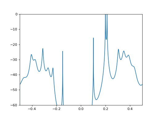
from spectrum import arma2psd, ma, marple_data
import pylab

# Estimate 15 Ma parameters
b, rho = ma(marple_data, 15, 30)
# Create the PSD from those MA parameters
psd = arma2psd(B=b, rho=rho, sides='centerdc')
# and finally plot the PSD
pylab.plot(pylab.linspace(-0.5, 0.5, 4096), 10 * pylab.log10(psd/max(psd)))
pylab.axis([-0.5, 0.5, -30, 0])
(
Source code,png,hires.png,pdf)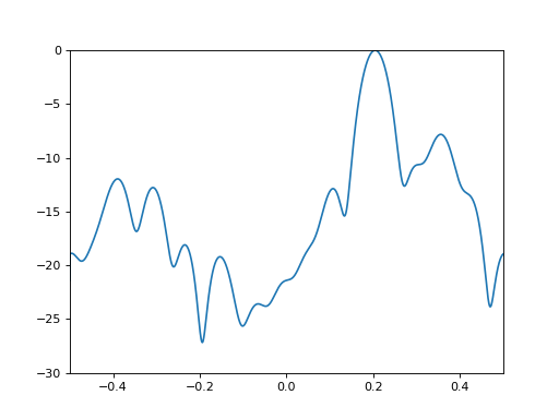
- Reference:
- class parma(data, P, Q, lag, NFFT=None, sampling=1.0, scale_by_freq=False)[source]
Class to create PSD using ARMA estimator.
See
arma_estimate()for description.from spectrum import parma, marple_data p = parma(marple_data, 4, 4, 30, NFFT=4096) p.plot(sides='centerdc')
(
Source code,png,hires.png,pdf)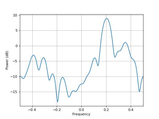
Constructor:
For a detailed description of the parameters, see
arma_estimate().
- class pma(data, Q, M, NFFT=None, sampling=1.0, scale_by_freq=False)[source]
Class to create PSD using MA estimator.
See
ma()for description.from spectrum import pma, marple_data p = pma(marple_data, 15, 30, NFFT=4096) p.plot(sides='centerdc')
(
Source code,png,hires.png,pdf)
Constructor:
For a detailed description of the parameters, see
ma().
5.3.1.2. AR estimate based on Burg algorithm
BURG method of AR model estimate
- arburg(X, order, criteria=None)[source]
Estimate the complex autoregressive parameters by the Burg algorithm.
- Parameters:
x – Array of complex data samples (length N)
order – Order of autoregressive process (0<order<N)
criteria – select a criteria to automatically select the order
- Returns:
A Array of complex autoregressive parameters A(1) to A(order). First value (unity) is not included !!
P Real variable representing driving noise variance (mean square of residual noise) from the whitening operation of the Burg filter.
reflection coefficients defining the filter of the model.
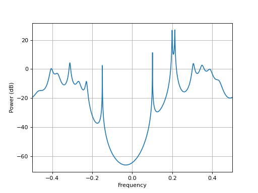
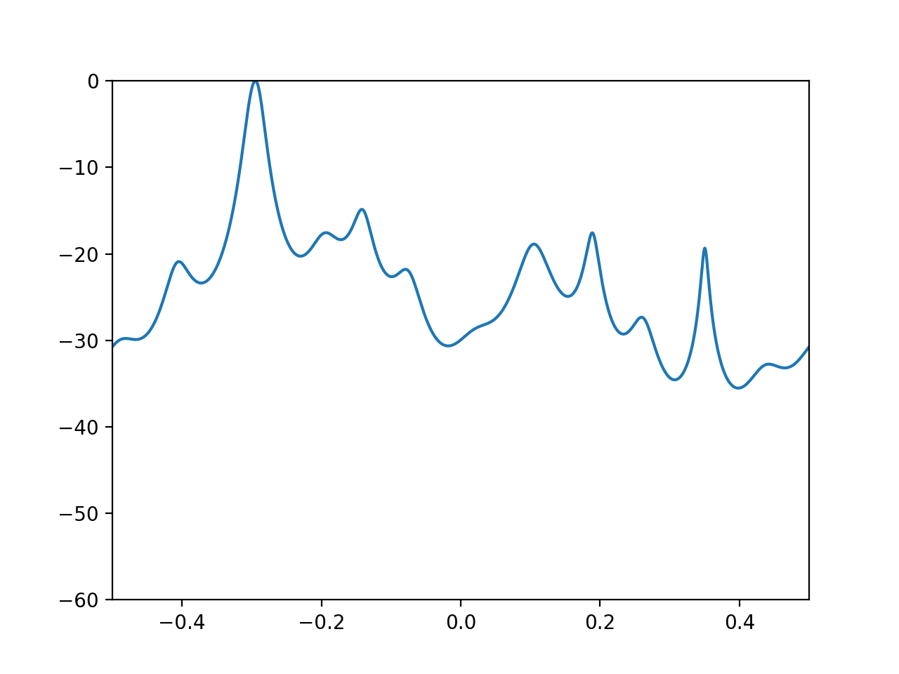
from pylab import plot, log10, linspace, axis
from spectrum import *

AR, P, k = arburg(marple_data, 15)
PSD = arma2psd(AR, sides='centerdc')
plot(linspace(-0.5, 0.5, len(PSD)), 10*log10(PSD/max(PSD)))
axis([-0.5,0.5,-60,0])
(
Source code,png,hires.png,pdf)
Note
no detrend. Should remove the mean trend to get PSD. Be careful if presence of large mean.
If you don’t know what the order value should be, choose the criterion=’AKICc’, which has the least bias and best resolution of model-selection criteria.
Note
real and complex results double-checked versus octave using complex 64 samples stored in marple_data. It does not agree with Marple fortran routine but this is due to the simplex precision of complex data in fortran.
- class pburg(data, order, criteria=None, NFFT=None, sampling=1.0, scale_by_freq=False)[source]
Class to create PSD based on Burg algorithm
See
arburg()for description.from spectrum import * p = pburg(marple_data, 15, NFFT=4096) p.plot(sides='centerdc')
(
Source code,png,hires.png,pdf)
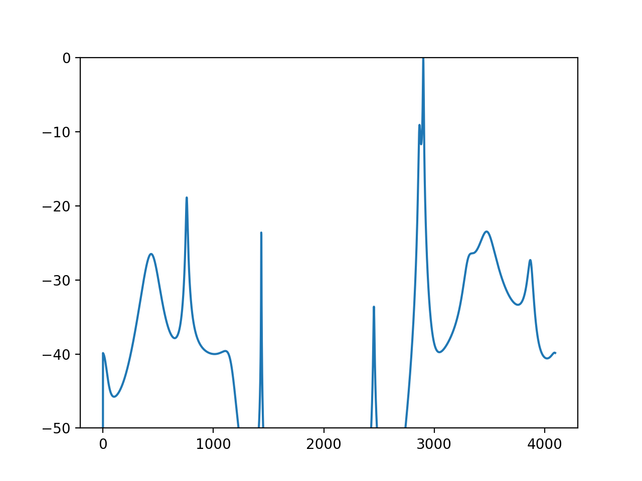
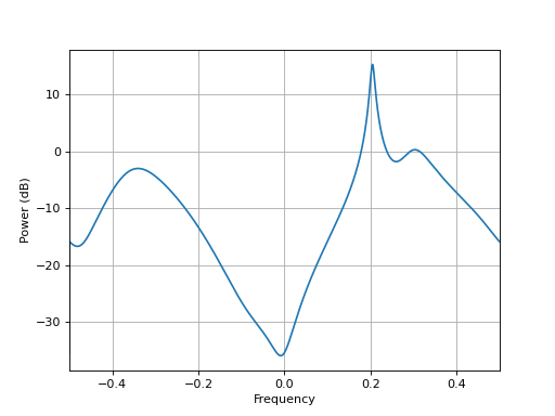
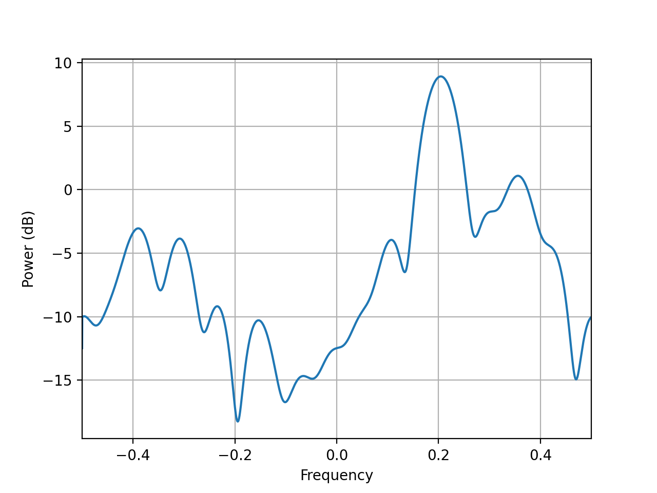
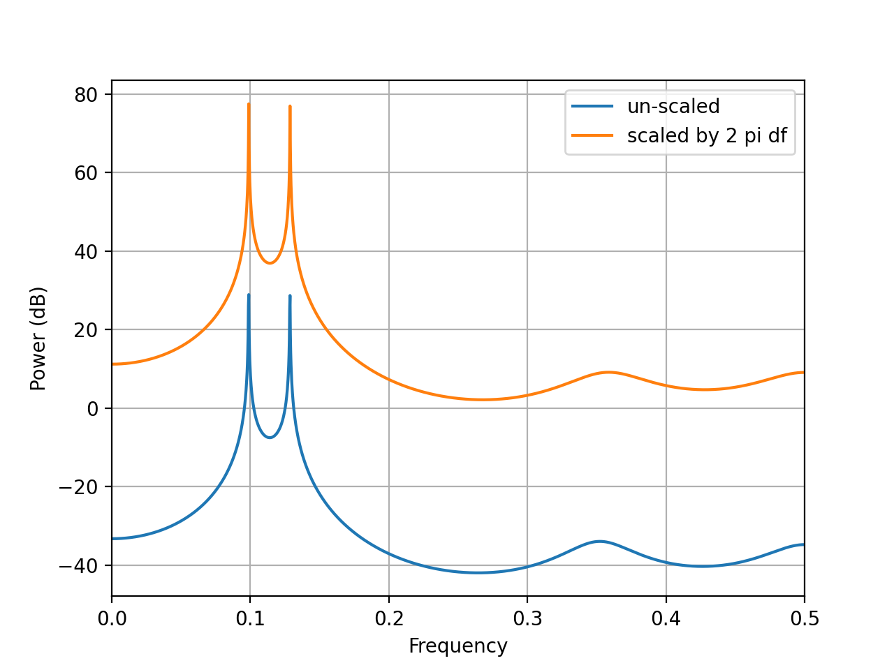
Another example based on a real data set is shown here below. Note here that we set the scale_by_freq value to False and True. False should give results equivalent to octave or matlab convention while setting to True implies that the data is multiplied by
 where
where
 .
.from spectrum import data_two_freqs, pburg p = pburg(data_two_freqs(), 7, NFFT=4096) p.plot() p = pburg(data_two_freqs(), 7, NFFT=4096, scale_by_freq=True) p.plot() from pylab import legend legend(["un-scaled", "scaled by 2 pi df"])
(
Source code,png,hires.png,pdf)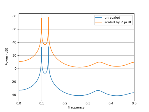
Constructor
For a detailled description of the parameters, see
burg().
5.3.1.3. AR estimate based on YuleWalker
Yule Walker method to estimate AR values.
- aryule(X, order, norm='biased', allow_singularity=True)[source]
Compute AR coefficients using Yule-Walker method
- Parameters:
- Returns:
AR coefficients (complex)
variance of white noise (Real)
reflection coefficients for use in lattice filter
Description:
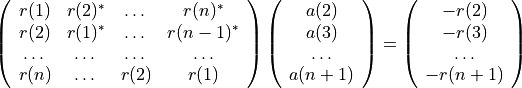
The Yule-Walker method returns the polynomial A corresponding to the AR parametric signal model estimate of vector X using the Yule-Walker (autocorrelation) method. The autocorrelation may be computed using a biased or unbiased estimation. In practice, the biased estimate of the autocorrelation is used for the unknown true autocorrelation. Indeed, an unbiased estimate may result in nonpositive-definite autocorrelation matrix. So, a biased estimate leads to a stable AR filter. The following matrix form represents the Yule-Walker equations. The are solved by means of the Levinson-Durbin recursion:
The outputs consists of the AR coefficients, the estimated variance of the white noise process, and the reflection coefficients. These outputs can be used to estimate the optimal order by using
criteria.Examples:
From a known AR process or order 4, we estimate those AR parameters using the aryule function.
>>> from scipy.signal import lfilter
>>> from spectrum import *
>>> from numpy.random import randn
>>> A  =[1, -2.7607, 3.8106, -2.6535, 0.9238]
>>> noise = randn(1, 1024)
>>> y = lfilter([1], A, noise);
>>> #filter a white noise input to create AR(4) process
>>> [ar, var, reflec] = aryule(y[0], 4)
>>> # ar should contains values similar to A
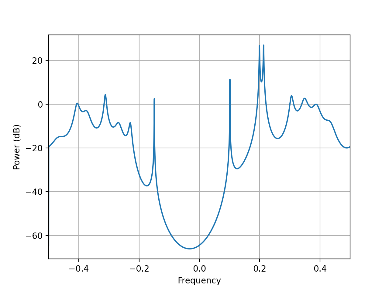
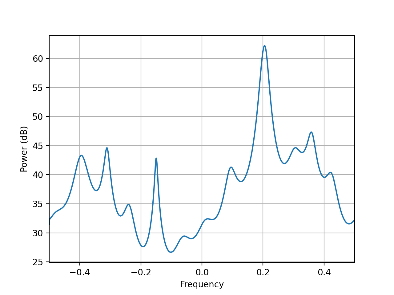
The PSD estimate of a data samples is computed and plotted as follows:
from spectrum import *
from pylab import *

ar, P, k = aryule(marple_data, 15, norm='biased')
psd = arma2psd(ar)
plot(linspace(-0.5, 0.5, 4096), 10 * log10(psd/max(psd)))
axis([-0.5, 0.5, -60, 0])
(
Source code,png,hires.png,pdf)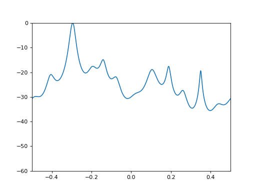
Note
The outputs have been double checked against (1) octave outputs (octave has norm=’biased’ by default) and (2) Marple test code.
See also
This function uses
LEVINSON()andCORRELATION(). See thecriteriamodule for criteria to automatically select the AR order.- References:
- class pyule(data, order, norm='biased', NFFT=None, sampling=1.0, scale_by_freq=True)[source]
Class to create PSD based on the Yule Walker method
See
aryule()for description.from spectrum import * p = pyule(marple_data, 15, NFFT=4096) p.plot(sides='centerdc')
(
Source code,png,hires.png,pdf)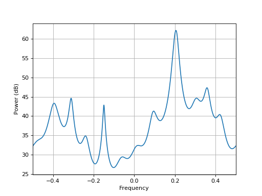
Constructor
For a detailled description of the parameters, see
aryule().
5.3.2. Criteria
Criteria for parametric methods.
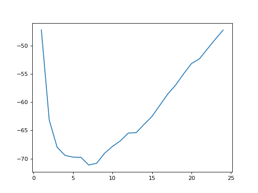
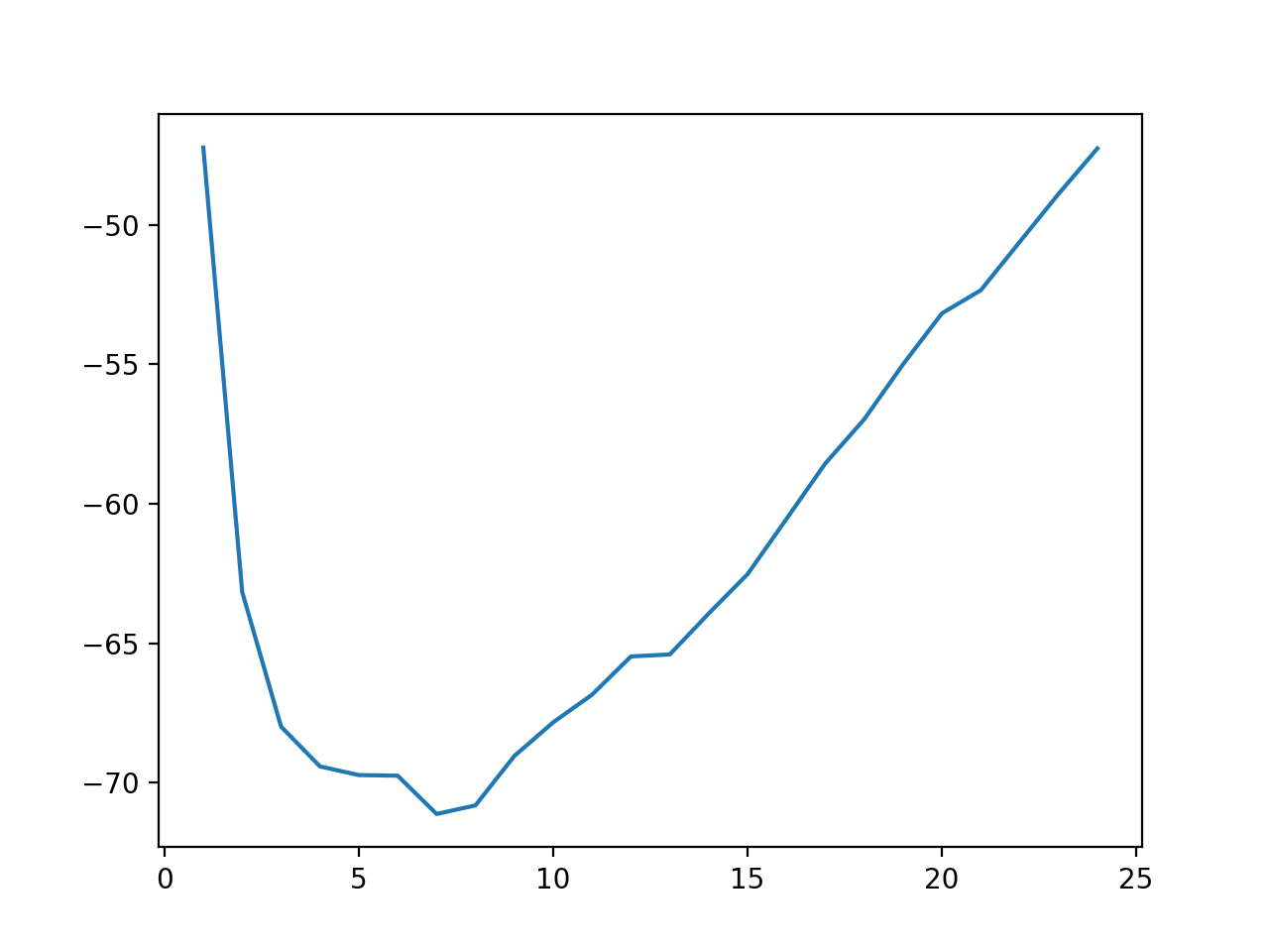
Example
from spectrum import aryule, AIC, marple_data
from pylab import plot, arange
order = arange(1, 25)
rho = [aryule(marple_data, i, norm='biased')[1] for i in order]
plot(order, AIC(len(marple_data), rho, order), label='AIC')
(Source code, png, hires.png, pdf)

- References:
bd-Krim Seghouane and Maiza Bekara “A small sample model selection criterion based on Kullback’s symmetric divergence”, IEEE Transactions on Signal Processing, Vol. 52(12), pp 3314-3323, Dec. 2004
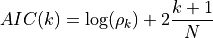
- AIC(N, rho, k)[source]
Akaike Information Criterion
- Parameters:
rho – rho at order k
N – sample size
k – AR order.
If k is the AR order and N the size of the sample, then Akaike criterion is
AIC(64, [0.5,0.3,0.2], [1,2,3])
- Validation:
double checked versus octave.
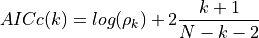
- AICc(N, rho, k, norm=True)[source]
corrected Akaike information criterion
- Validation:
double checked versus octave.

- class Criteria(name, N)[source]
Criteria class for an automatic selection of ARMA order.
Available criteria are
AIC
see
AIC()AICc
see
AICc()KIC
see
KIC()AKICc
see
AKICc()FPE
see
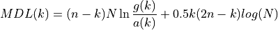
FPE()MDL
see
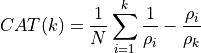
MDL()CAT
see
_CAT()Create a criteria object
- Parameters:
name – a string or list of strings containing valid criteria method’s name
N (int) – size of the data sample.
- property N
Getter/Setter for N
- property data
Getter/Setter for the criteria output
- error_incorrect_name = "Invalid name provided. Correct names are ['AIC', 'AICc', 'KIC', 'FPE', 'AKICc', 'MDL'] "
- error_no_criteria_found = "No names match the valid criteria names (['AIC', 'AICc', 'KIC', 'FPE', 'AKICc', 'MDL'])"
- property k
Getter for k the order of evaluation
- property name
Getter/Setter for the criteria name
- property old_data
Getter/Setter for the previous value
- property rho
Getter/Setter for rho
- valid_criteria_names = ['AIC', 'AICc', 'KIC', 'FPE', 'AKICc', 'MDL']
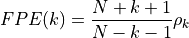
- FPE(N, rho, k=None)[source]
Final prediction error criterion
- Validation:
double checked versus octave.

- aic_eigen(s, N)[source]
AIC order-selection using eigen values
- Parameters:
s – a list of p sorted eigen values
N – the size of the input data. To be defined precisely.
- Returns:
an array containing the AIC values
Given
 sorted eigen values
  with
with
 , the proposed criterion from Wax and Kailath (1985)
is:
, the proposed criterion from Wax and Kailath (1985)
is: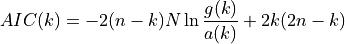
where the arithmetic sum
 is:
is: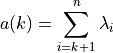
and the geometric sum
 is:
is: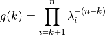
The number of relevant sinusoids in the signal subspace is determined by selecting the minimum of AIC.
See also
eigen()Todo
define precisely the input parameter N. Should be the input data length but when using correlation matrix (SVD), I suspect it should be the length of the correlation matrix rather than the original data.
- mdl_eigen(s, N)[source]
MDL order-selection using eigen values
- Parameters:
s – a list of p sorted eigen values
N – the size of the input data. To be defined precisely.
- Returns:
an array containing the AIC values
See also
aic_eigen()for details