5.5. Tools and classes ¶

5.5.1. Classes ¶

This module provides the Base class for PSDs

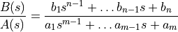
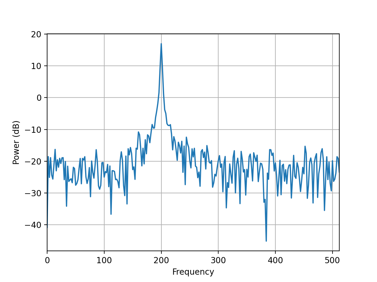
class FourierSpectrum(data, sampling=1.0, window='hanning', NFFT=None, detrend=None, scale_by_freq=True, lag=-1)[source]¶

Spectrum based on Fourier transform.

This class inherits attributes and methods from Spectrum. It is used by children class Periodogram, pcorrelogram and Welch PSD estimates.

The parameters are those used by Spectrum

Parameters:

data (array) – Input data (list or numpy.array)
data_y – input data required to perform cross-PSD only.
sampling (float) – sampling frequency of the input data
detrend (str) – detrend method ([None,’mean’]) to apply on the input data before computing the PSD. See detrend.
scale_by_freq (bool) – Divide the final PSD by $2*\pi/df$
NFFT (int) – total length of the data given to the FFT

In addition you need specific parameters such as:

Parameters:

window (str) – a tapering window. See Window.
lag (int) – to be used by the pcorrelogram methods only.

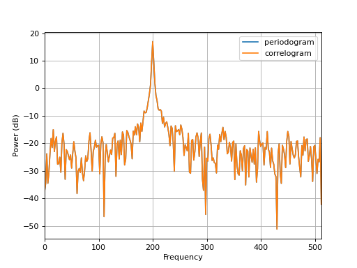
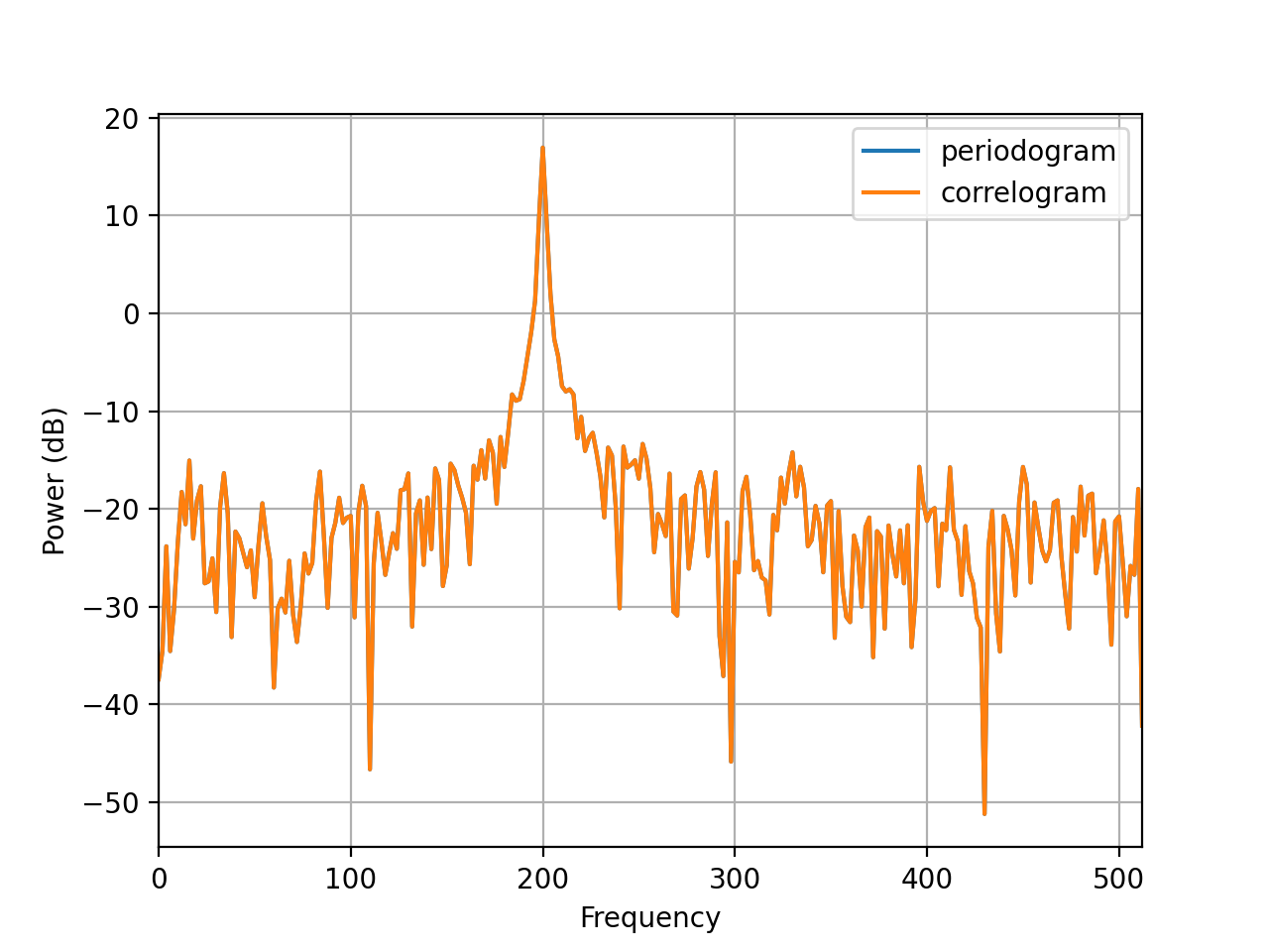
This class has dedicated PSDs methods such as speriodogram(), which are equivalent to children class such as Periodogram.

from spectrum import datasets
from spectrum import FourierSpectrum
s = FourierSpectrum(datasets.data_cosine(), lag=32, sampling=1024, NFFT=512)
s.periodogram()
s.plot(label='periodogram')
#s.correlogram()
s.plot(label='correlogram')
from pylab import legend, xlim
legend()
xlim(0,512)

(Source code, png, hires.png, pdf)

Constructor

See the class documentation for the parameters.

Additional attributes to those inherited from

Spectrum are:

lag, a lag used to compute the autocorrelation
window, the tapering window to be used

property lag¶: Getter/Setter used by the correlogram when autocorrelation estimates are required.

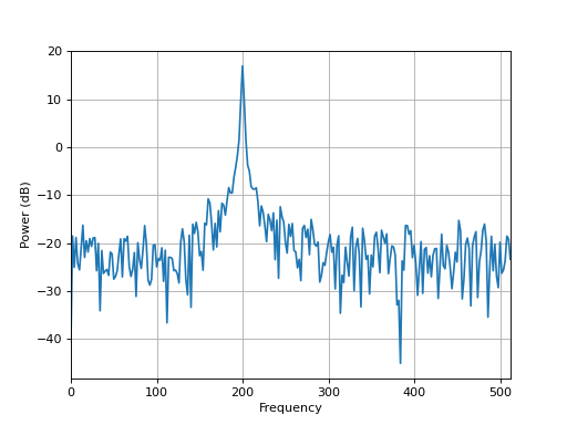
periodogram()[source]¶

An alias to Periodogram

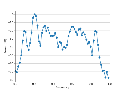
The parameters are extracted from the attributes. Relevant attributes ares window, attr:sampling, attr:NFFT, attr:scale_by_freq, detrend.

from spectrum import datasets
from spectrum import FourierSpectrum
s = FourierSpectrum(datasets.data_cosine(), sampling=1024, NFFT=512)
s.periodogram()
s.plot()

(Source code, png, hires.png, pdf)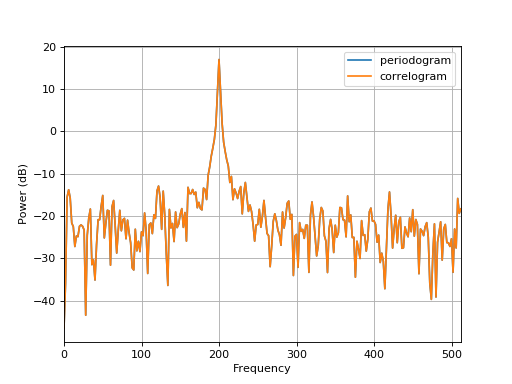

property window¶: Tapering window to be applied

class ParametricSpectrum(data, sampling=1.0, ar_order=None, ma_order=None, lag=-1, NFFT=None, detrend=None, scale_by_freq=True)[source]¶

Spectrum based on Fourier transform.

This class inherits attributes and methods from Spectrum. It is used by children class Periodogram, pcorrelogram and Welch PSD estimates. The parameters are those used by Spectrum.

Parameters:

data (array) – Input data (list or numpy.array)
sampling (float) – sampling frequency of the input data
detrend (str) – detrend method ([None,’mean’]) to apply on the input data before computing the PSD. See detrend.
scale_by_freq (bool) – Divide the final PSD by $2*\pi/df$

In addition you need specific parameters such as:

Parameters:

window (str) – a tapering window. See Window.
lag (int) – to be used by the pcorrelogram methods only.
NFFT (int) – Total length of the data given to the FFT

This class has dedicated PSDs methods such as periodogram(), which are equivalent to children class such as Periodogram.

from spectrum import datasets
from spectrum import ParametricSpectrum
data = datasets.data_cosine(N=1024)
s = ParametricSpectrum(data, ar_order=4, ma_order=4, sampling=1024, NFFT=512, lag=10)
#s.parma()
#s.plot(sides='onesided')
#s.plot(sides='twosided')

(Source code)

Constructor

See the class documentation for the parameters.

Additional attributes to those inherited from Spectrum:

ar_order, the ar order of the PSD estimates
ma_order, the ar order of the PSD estimates

property ar¶

property ar_order¶

property ma¶

property ma_order¶

plot_reflection()[source]¶

property reflection¶: Reflection coefficients of the AR model.

property rho¶

class Range(N, sampling=1.0)[source]¶

A class to ease the creation of frequency ranges.

Given the length N of a data sample and a sampling frequency sampling, this class provides methods to generate frequency ranges

centerdc(): frequency range from -sampling/2 up to sampling/2 (excluded),

twosided(): frequency range from 0 up to sampling (excluded),

onesided(): frequency range from 0 up to sampling (included or excluded depending on evenness of the data). If NFFT is even, PSD has length NFFT/2 + 1 over the interval [0,pi]. If NFFT is odd, the length of PSD is (NFFT+1)/2 and the interval is [0, pi)

Each method has a generator version:

>>> r = Range(10, sampling=1)
>>> list(r.onesided_gen())
[0.0, 0.1, 0.2, 0.3, 0.4, 0.5]
>>> r.onesided()
[0.0, 0.1, 0.2, 0.3, 0.4, 0.5]

The frequency range length is $N/2+1$ for the onesided case $((N+1)/2$ if $N$ is odd), and $N$ for the twosided and centerdc cases:

>>> r.twosided()
[0.0, 0.1, 0.2, 0.3, 0.4, 0.5, 0.6, 0.7, 0.8, 0.9]
>>> len(r.twosided())
10
>>> len(r.centerdc())
10
>>> len(r.onesided())
5

Constructor

Parameters:

N (int) – the data length
sampling (float) – sampling frequency of the input data.

Attributes:

From the input parameters, read/write attributes are set:

N, the data length,

sampling, the sampling frequency.

Additionally, the following read-only attribute is available:

df, the frequency step computed from N and sampling.

property N¶: Getter/Setter of the data length. If changed, df is updated.

centerdc()[source]¶: Return the two-sided frequency range as a list (see centerdc_gen() for details).

centerdc_gen()[source]¶

Return the centered frequency range as a generator.

>>> print(list(Range(8).centerdc_gen()))
[-0.5, -0.375, -0.25, -0.125, 0.0, 0.125, 0.25, 0.375]

property df¶: Getter to access the frequency step, computed from N and sampling.

onesided()[source]¶: Return the one-sided frequency range as a list (see onesided_gen() for details).

onesided_gen()[source]¶

Return the one-sided frequency range as a generator.

If N is even, the length is N/2 + 1. If N is odd, the length is (N+1)/2.

>>> print(list(Range(8).onesided()))
[0.0, 0.125, 0.25, 0.375, 0.5]
>>> print(list(Range(9).onesided()))
[0.0, 0.1111, 0.2222, 0.3333, 0.4444]

property sampling¶: Getter/Setter of the sampling frequency. If changed, df is updated.

twosided()[source]¶: Return the two-sided frequency range as a list (see twosided_gen() for details).

twosided_gen()[source]¶

Returns the twosided frequency range as a generator

>>> print(list(Range(8).centerdc_gen()))
[0, 0.125, 0.25, 0.375, 0.5, 0.625, 0.75, 0.875]

class Spectrum(data, data_y=None, sampling=1.0, detrend=None, scale_by_freq=True, NFFT=None)[source]¶

Base class for all Spectrum classes

All PSD classes should inherits from this class to store common attributes such as the input data or sampling frequency. An instance is created as follows:

>>> p = Spectrum(data, sampling=1024)
>>> p.data
>>> p.sampling

The input parameters are:

Parameters:

data (array) – input data (list or numpy.array)
data_y (array) – input data required to perform cross-PSD only.
sampling (float) – sampling frequency of the input data
detrend (str) – detrend method ([None,’mean’]) to apply on the input data before computing the PSD. See detrend.
scale_by_freq (bool) – divide the final PSD by $2*\pi/df$
NFFT (int) – total length of the final data sets (padded with zero if needed; default is 4096)

The input parameters are available as attributes. Additional attributes such as N (the data length), df (the frequency step are set (see constructor documentation for a complete list).

Warning

Spectrum does not compute the PSD estimate.

You can populate manually the psd attribute but you should respect the following convention:

if the input data is real, the PSD is assumed to be one-sided (odd length)

if the input data is complex, the PSD is assumed to be two-sided (even length).

When psd is set, sides is reset to its default value, NFFT and df are updated.

Spectrum instances have plotting utilities like plot() that take care of plotting the PSD versus the appropriate frequency range (based on sampling, NFFT and sides)

Note

the modification of some attributes (e.g., NFFT), makes the PSD obsolete. In such cases, the PSD must be re-computed before using plot() again.

At any time, you can get general information about the Spectrum instance:

>>> p = Spectrum(marple_data)
>>> print(p)
Spectrum summary
    Data length is 64
    PSD not yet computed
    Sampling 1.0
    freq resolution 0.015625
    datatype is complex
    sides is twosided
    scal_by_freq is True

Constructor

Attributes:

From the input parameters, the following attributes are set:

data (updates N, df, datatype)

data_y used for cross PSD only (correlogram)

detrend

sampling (updates df)

scale_by_freq

NFFT (reset sides, df)

The following read-only attributes are set during the initialisation:

datatype

df

N

And finally, additional read-write attributes are available:

psd: used to store the PSD data array, which size depends on sides i.e., one-sided for real data and two-sided for the complex data.

sides: if set, changed the psd.

property N¶: Getter to the original data size. N is automatically updated when changing the data only.

property NFFT¶

Getter/Setter to the NFFT attribute.

Parameters:

NFFT –

a user choice for setting NFFT.

if None, the NFFT is set to N, the data length.
if ‘nextpow2’, computes the next power of 2 greater than or equal to the data length.
if a integer is provided, it must be positive

If NFFT is changed, sides is reset and df as well.

property data¶: Getter/Setter for the input data. If input is a list, it is cast into a numpy.array. Then, N, df and datatype are updated.

property data_y¶: Getter/Setter to the Y-data

property datatype¶: Getter to the datatype (‘real’ or ‘complex’). datatype is automatically updated when changing the data.

property detrend¶

Getter/Setter to detrend:

None: do not perform any detrend.
‘mean’: remove the mean value of each segment from each segment of the data.
‘long-mean’: remove the mean value from the data before splitting it into segments.
‘linear’: remove linear trend from each segment.

property df¶: Getter to step frequency. This attribute is updated as soon as data or sampling is changed

frequencies(sides=None)[source]¶: Return the frequency vector according to sides

get_converted_psd(sides)[source]¶

This function returns the PSD in the sides format

Parameters:: sides (str) – the PSD format in [‘onesided’, ‘twosided’, ‘centerdc’]
Returns:: the expected PSD.

from spectrum import *
p = pcovar(marple_data, 15)
centerdc_psd = p.get_converted_psd('centerdc')

Note

this function does not change the object, in particular, it does not change the psd attribute. If you want to change the psd on the fly, change the attribute sides.

property method¶: The PSD estimation method (alias to the class name).

plot(filename=None, norm=False, ylim=None, sides=None, **kargs)[source]¶

a simple plotting routine to plot the PSD versus frequency.

Parameters:

filename (str) – save the figure into a file
norm – False by default. If True, the PSD is normalised.
ylim – readjust the y range .
sides – if not provided, sides is used. See sides for details.
kargs – any optional argument accepted by pylab.plot().

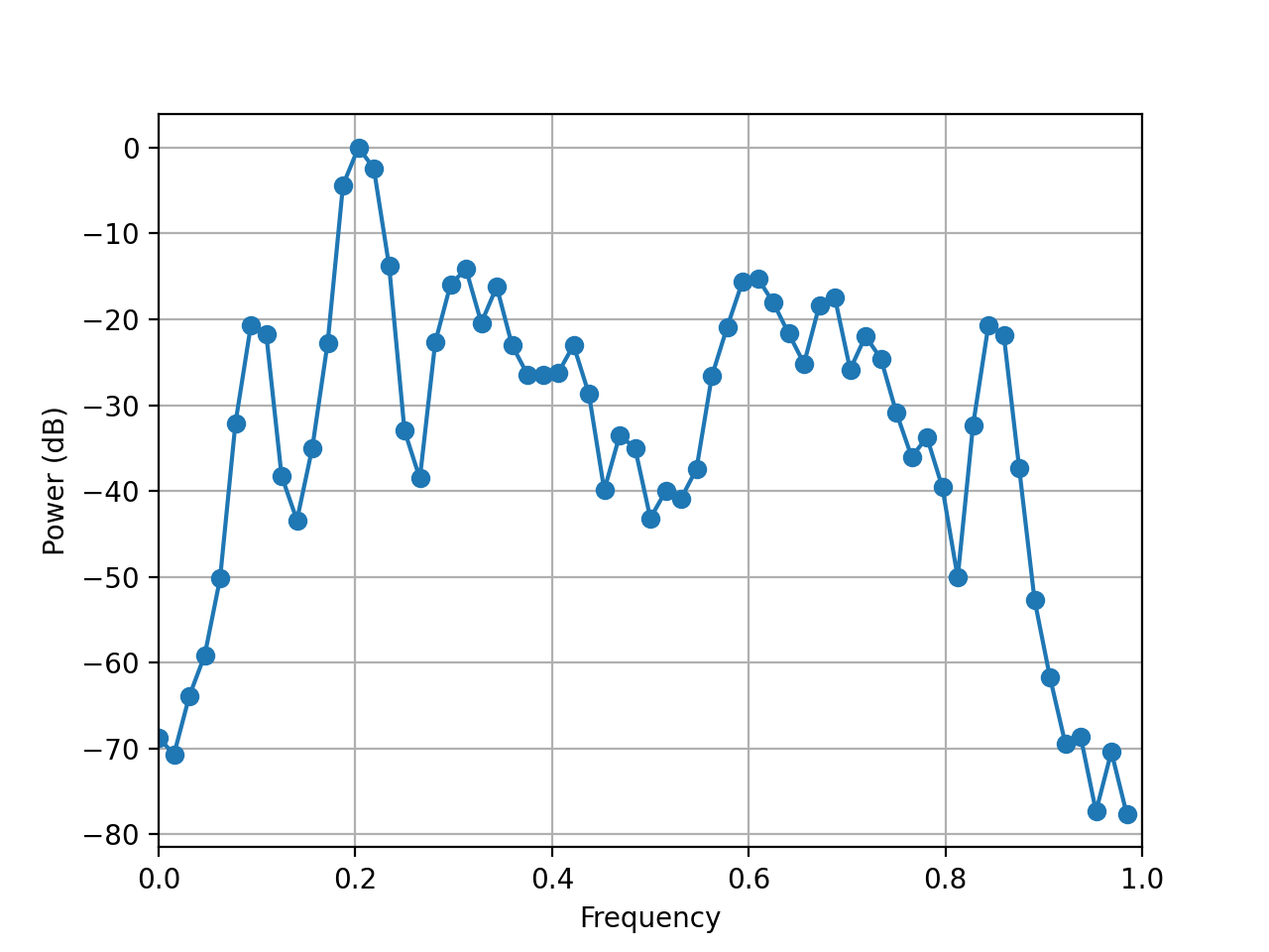
from spectrum import *
p = Periodogram(marple_data)
p.plot(norm=True, marker='o')

(Source code, png, hires.png, pdf)

power()[source]¶

Return the power contained in the PSD

if scale_by_freq is False, the power is:

$P = N \sum_{k=1}^{N} P_{xx}(k)$

else, it is

$P = \sum_{k=1}^{N} P_{xx}(k) \frac{df}{2\pi}$

Todo

check these equations

property psd¶

Getter/Setter to psd

Parameters:: psd (array) – the array must be in agreement with the onesided/twosided convention: if the data in real, the psd must be onesided. If the data is complex, the psd must be twosided.

When you set this attribute, several attributes are set:

sides is set to onesided if datatype is real and twosided if datatype is complex.

NFFT is set to len(psd)*2 if sides=onesided and (len(psd)-1)*2 if sides=twosided.

range.N is set to NFFT, which update df.

property range¶: Read only attribute to a Range object.

run(*args, **kargs)[source]¶

property sampling¶: Getter/Setter to sampling frequency. Updates the df automatically.

scale()[source]¶

property scale_by_freq¶: scale the PSD by $2*\pi/df$

property sides¶

Getter/Setter to the sides attributes.

It can be ‘onesided’, ‘twosided’, ‘centerdc’. This setter changes psd to reflect the user argument choice.

If the datatype is complex, sides cannot be one-sided.

5.5.2. Correlation ¶

CORRELATION(x, y=None, maxlags=None, norm='unbiased')[source]¶

Correlation function

This function should give the same results as xcorr() but it returns the positive lags only. Moreover the algorithm does not use FFT as compared to other algorithms.

Parameters:

x (array) – first data array of length N
y (array) – second data array of length N. If not specified, computes the autocorrelation.
maxlags (int) – compute cross correlation between [0:maxlags] when maxlags is not specified, the range of lags is [0:maxlags].
norm (str) –
normalisation in [‘biased’, ‘unbiased’, None, ‘coeff’]
- biased correlation=raw/N,
- unbiased correlation=raw/(N-|lag|)
- coeff correlation=raw/(rms(x).rms(y))/N
- None correlation=raw

Returns:

a numpy.array correlation sequence, r[1,N]
a float for the zero-lag correlation, r[0]

The unbiased correlation has the form:

$\hat{r}_{xx} = \frac{1}{N-m}T \sum_{n=0}^{N-m-1} x[n+m]x^*[n] T$

The biased correlation differs by the front factor only:

$\check{r}_{xx} = \frac{1}{N}T \sum_{n=0}^{N-m-1} x[n+m]x^*[n] T$

with $0\leq m\leq N-1$ .

>>> from spectrum import CORRELATION
>>> x = [1,2,3,4,5]
>>> res = CORRELATION(x,x, maxlags=0, norm='biased')
>>> res[0]
11.0

Note

this function should be replaced by xcorr().

See also

xcorr()

xcorr(x, y=None, maxlags=None, norm='biased')[source]¶

Cross-correlation using numpy.correlate

Estimates the cross-correlation (and autocorrelation) sequence of a random process of length N. By default, there is no normalisation and the output sequence of the cross-correlation has a length 2*N+1.

Parameters:

x (array) – first data array of length N
y (array) – second data array of length N. If not specified, computes the autocorrelation.
maxlags (int) – compute cross correlation between [-maxlags:maxlags] when maxlags is not specified, the range of lags is [-N+1:N-1].
option (str) – normalisation in [‘biased’, ‘unbiased’, None, ‘coeff’]

The true cross-correlation sequence is

$r_{xy}[m] = E(x[n+m].y^*[n]) = E(x[n].y^*[n-m])$

However, in practice, only a finite segment of one realization of the infinite-length random process is available.

The correlation is estimated using numpy.correlate(x,y,’full’). Normalisation is handled by this function using the following cases:

‘biased’: Biased estimate of the cross-correlation function

‘unbiased’: Unbiased estimate of the cross-correlation function

‘coeff’: Normalizes the sequence so the autocorrelations at zero
lag is 1.0.

Returns:

a numpy.array containing the cross-correlation sequence (length 2*N-1)
lags vector

Note

If x and y are not the same length, the shorter vector is zero-padded to the length of the longer vector.

Examples

>>> from spectrum import xcorr
>>> x = [1,2,3,4,5]
>>> c, l = xcorr(x,x, maxlags=0, norm='biased')
>>> c
array([ 11.])

See also

CORRELATION().

5.5.3. Tools ¶

centerdc_2_twosided(data)[source]¶: Convert a center-dc PSD to a twosided PSD

cshift(data, offset)[source]¶

Circular shift to the right (within an array) by a given offset

Parameters:

data (array) – input data (list or numpy.array)
offset (int) – shift the array with the offset

>>> from spectrum import cshift
>>> cshift([0, 1, 2, 3, -2, -1], 2)
array([-2, -1,  0,  1,  2,  3])

db2mag(xdb)[source]¶

Convert decibels (dB) to magnitude

>>> from spectrum import db2mag
>>> db2mag(-20)
0.1

See also

pow2db()

db2pow(xdb)[source]¶

Convert decibels (dB) to power

>>> from spectrum import db2pow
>>> p = db2pow(-10)
>>> p
0.1

See also

pow2db()

fftshift(x)[source]¶

wrapper to numpy.fft.fftshift

>>> from spectrum import fftshift
>>> x = [100, 2, 3, 4, 5]
>>> fftshift(x)
array([  4,   5, 100,   2,   3])

log10(data)[source]¶

mag2db(x)[source]¶

Convert magnitude to decibels (dB)

The relationship between magnitude and decibels is:

$X_{dB} = 20 * \log_{10}(x)$

>>> from spectrum import mag2db
>>> mag2db(0.1)
-20.0

See also

db2mag()

nextpow2(x)[source]¶

returns the smallest power of two that is greater than or equal to the absolute value of x.

This function is useful for optimizing FFT operations, which are most efficient when sequence length is an exact power of two.

Example:

>>> from spectrum import nextpow2
>>> x = [255, 256, 257]
>>> nextpow2(x)
array([8, 8, 9])

onesided_2_twosided(data)[source]¶

Convert a two-sided PSD to a one-sided PSD

In order to keep the power in the twosided PSD the same as in the onesided version, the twosided values are 2 times lower than the input data (except for the zero-lag and N-lag values).

>>> twosided_2_onesided([10, 4, 6, 8])
array([ 10.,   2.,   3.,   3., 2., 8.])

pow2db(x)[source]¶

returns the corresponding decibel (dB) value for a power value x.

The relationship between power and decibels is:

$X_{dB} = 10 * \log_{10}(x)$

>>> from spectrum import pow2db
>>> x = pow2db(0.1)
>>> x
-10.0

twosided(data)[source]¶

return a twosided vector with non-duplication of the first element

>>> from spectrum import twosided
>>> a = [1,2,3]
>>> twosided(a)
array([3, 2, 1, 2, 3])

twosided_2_centerdc(data)[source]¶: Convert a two-sided PSD to a center-dc PSD

twosided_2_onesided(data)[source]¶

Convert a one-sided PSD to a twosided PSD

In order to keep the power in the onesided PSD the same as in the twosided version, the onesided values are twice as much as in the input data (except for the zero-lag value).

>>> twosided_2_onesided([10, 2,3,3,2,8])
array([ 10.,   4.,   6.,   8.])

5.5.4. datasets ¶

class TimeSeries(data, sampling=1)[source]¶

A simple Base Class for various data sets.

>>> from spectrum import TimeSeries
>>> data = [1, 2, 3, 4, 3, 2, 1, 0 ]
>>> ts = TimeSeries(data, sampling=1)
>>> ts.plot()
>>> ts.dt
1.0

Parameters:

data (array) – input data (list or numpy.array)
sampling – the sampling frequency of the data (default 1Hz)

plot(**kargs)[source]¶: Plot the data set, using the sampling information to set the x-axis correctly.

data_cosine(N=1024, A=0.1, sampling=1024.0, freq=200)[source]¶

Return a noisy cosine at a given frequency.

Parameters:

N – the final data size
A – the strength of the noise
sampling (float) – sampling frequency of the input data.
freq (float) – the frequency $f_0$ of the cosine.

$x[t] = cos(2\pi t * f_0) + A w[t]$

where w[t] is a white noise of variance 1.

>>> from spectrum import data_cosine
>>> a = data_cosine(N=1024, sampling=1024, A=0.5, freq=100)

data_two_freqs(N=200)[source]¶: A simple test example with two close frequencies

dolphin_filename = '/home/docs/checkouts/readthedocs.org/user_builds/pyspectrum/envs/stable/lib/python3.10/site-packages/spectrum/data/DOLPHINS.wav'¶: filename of a WAV data file 150,000 data points

marple_data = [(1.349839091+2.011167288j), (-2.117270231+0.817693591j), (-1.786421657-1.291698933j), (1.162236333-1.482598066j), (1.641072035+0.372950256j), (0.072213709+1.828492761j), (-1.564284801+0.824533045j), (-1.080565453-1.869776845j), (0.92712909-1.743406534j), (1.891979456+0.972347319j), (-0.105391249+1.602209687j), (-1.618367076+0.63751328j), (-0.945704579-1.079569221j), (1.135566235-1.692269921j), (1.855816245+0.986030221j), (-1.032083511+1.414613724j), (-1.571600199+0.089229003j), (-0.243143231-1.444692016j), (0.838980973-0.985756695j), (1.516003132+0.928058863j), (0.257979959+1.170676708j), (-2.057927608+0.343388647j), (-0.578682184-1.441192508j), (1.584011555-1.011150956j), (0.614114344+1.508176208j), (-0.710567117+1.130144477j), (-1.100205779-0.584209621j), (0.150702029-1.217450142j), (0.748856127-0.804411888j), (0.795235813+1.114466429j), (-0.071512341+1.017092347j), (-1.732939839-0.283070654j), (0.404945314-0.78170836j), (1.293794155-0.352723092j), (-0.119905084+0.905150294j), (-0.522588372+0.437393665j), (-0.974838495-0.670074046j), (0.275279552-0.509659231j), (0.854210198-0.008278057j), (0.289598197+0.50623399j), (-0.283553183+0.250371397j), (-0.359602571-0.135261074j), (0.102775671-0.466086507j), (-0.00972265+0.030377999j), (0.185930878+0.8088696j), (-0.243692726-0.200126961j), (-0.270986766-0.460243553j), (0.399368525+0.249096692j), (-0.250714004-0.36299023j), (0.419116348-0.389185309j), (-0.050458215+0.702862442j), (-0.395043731+0.140808776j), (0.746575892-0.126762003j), (-0.55907619+0.523169816j), (-0.34438926-0.913451135j), (0.733228028-0.006237417j), (-0.480273813+0.509469569j), (0.033316225+0.087501869j), (-0.32122913-0.254548967j), (-0.063007891-0.499800682j), (1.239739418-0.013479125j), (0.083303742+0.673984587j), (-0.762731433+0.40897125j), (-0.895898521-0.364855707j)]¶: 64-complex data length from Marple reference [Marple]

spectrum_data(filename)[source]¶: Simple utilities to retrieve data sets from

5.5.5. Linear Algebra Tools ¶

5.5.5.1. cholesky ¶

CHOLESKY(A, B, method='scipy')[source]¶

Solve linear system AX=B using CHOLESKY method.

Parameters:

A – an input Hermitian matrix
B – an array
method (str) –
a choice of method in [numpy, scipy, numpy_solver]
- numpy_solver relies entirely on numpy.solver (no cholesky decomposition)
- numpy relies on the numpy.linalg.cholesky for the decomposition and numpy.linalg.solve for the inversion.
- scipy uses scipy.linalg.cholesky for the decomposition and scipy.linalg.cho_solve for the inversion.

Description

When a matrix is square and Hermitian (symmetric with lower part being the complex conjugate of the upper one), then the usual triangular factorization takes on the special form:

$A = R R^H$

where $R$ is a lower triangular matrix with nonzero real principal diagonal element. The input matrix can be made of complex data. Then, the inversion to find $x$ is made as follows:

$Ry = B$

and

$Rx = y$

>>> import numpy
>>> from spectrum import CHOLESKY
>>> A = numpy.array([[ 2.0+0.j ,  0.5-0.5j, -0.2+0.1j],
...    [ 0.5+0.5j,  1.0+0.j ,  0.3-0.2j],
...    [-0.2-0.1j,  0.3+0.2j,  0.5+0.j ]])
>>> B = numpy.array([ 1.0+3.j ,  2.0-1.j ,  0.5+0.8j])
>>> CHOLESKY(A, B)
array([ 0.95945946+5.25675676j,  4.41891892-7.04054054j,
       -5.13513514+6.35135135j])

5.5.5.2. eigen ¶

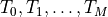
MINEIGVAL(T0, T, TOL)[source]¶

Finds the minimum eigenvalue of a Hermitian Toeplitz matrix

The classical power method is used together with a fast Toeplitz equation solution routine. The eigenvector is normalized to unit length.

Parameters:

T0 – Scalar corresponding to real matrix element t(0)
T – Array of M complex matrix elements t(1),…,t(M) C from the left column of the Toeplitz matrix
TOL – Real scalar tolerance; routine exits when [ EVAL(k) - EVAL(k-1) ]/EVAL(k-1) < TOL , where the index k denotes the iteration number.

Returns:

EVAL - Real scalar denoting the minimum eigenvalue of matrix
EVEC - Array of M complex eigenvector elements associated

Note

External array T must be dimensioned >= M
array EVEC must be >= M+1
Internal array E must be dimensioned >= M+1 .
dependencies
- spectrum.toeplitz.HERMTOEP()

5.5.5.3. levinson ¶

LEVINSON(r, order=None, allow_singularity=False)[source]¶

Levinson-Durbin recursion.

Find the coefficients of a length(r)-1 order autoregressive linear process

Parameters:

r – autocorrelation sequence of length N + 1 (first element being the zero-lag autocorrelation)
order – requested order of the autoregressive coefficients. default is N.
allow_singularity – false by default. Other implementations may be True (e.g., octave)

Returns:

the N+1 autoregressive coefficients $A=(1, a_1...a_N)$
the prediction errors
the N reflections coefficients values

This algorithm solves the set of complex linear simultaneous equations using Levinson algorithm.

$\bold{T}_M \left( \begin{array}{c} 1 \\ \bold{a}_M \end{array} \right) = \left( \begin{array}{c} \rho_M \\ \bold{0}_M \end{array} \right)$

where $\bold{T}_M$ is a Hermitian Toeplitz matrix with elements $T_0, T_1, \dots ,T_M$ .

Note

Solving this equations by Gaussian elimination would require $M^3$ operations whereas the levinson algorithm requires $M^2+M$ additions and $M^2+M$ multiplications.

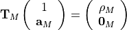
This is equivalent to solve the following symmetric Toeplitz system of linear equations

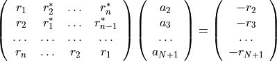
$\left( \begin{array}{cccc} r_1 & r_2^* & \dots & r_{n}^*\\ r_2 & r_1^* & \dots & r_{n-1}^*\\ \dots & \dots & \dots & \dots\\ r_n & \dots & r_2 & r_1 \end{array} \right) \left( \begin{array}{cccc} a_2\\ a_3 \\ \dots \\ a_{N+1} \end{array} \right) = \left( \begin{array}{cccc} -r_2\\ -r_3 \\ \dots \\ -r_{N+1} \end{array} \right)$

where $r = (r_1 ... r_{N+1})$ is the input autocorrelation vector, and $r_i^*$ denotes the complex conjugate of $r_i$ . The input r is typically a vector of autocorrelation coefficients where lag 0 is the first element $r_1$ .

>>> import numpy; from spectrum import LEVINSON
>>> T = numpy.array([3., -2+0.5j, .7-1j])
>>> a, e, k = LEVINSON(T)

rlevinson(a, efinal)[source]¶

computes the autocorrelation coefficients, R based on the prediction polynomial A and the final prediction error Efinal, using the stepdown algorithm.

Works for real or complex data

Parameters:

a
efinal

Returns:

R, the autocorrelation
U prediction coefficient
kr reflection coefficients
e errors

A should be a minimum phase polynomial and A(1) is assumed to be unity.

Returns:

(P+1) by (P+1) upper triangular matrix, U,: that holds the i’th order prediction polynomials Ai, i=1:P, where P is the order of the input polynomial, A.

[ 1 a1(1)* a2(2)* ….. aP(P) * ] [ 0 1 a2(1)* ….. aP(P-1)* ]
U = [ ……………………………]: [ 0 0 0 ….. 1 ]

from which the i’th order prediction polynomial can be extracted using Ai=U(i+1:-1:1,i+1)’. The first row of U contains the conjugates of the reflection coefficients, and the K’s may be extracted using, K=conj(U(1,2:end)).

Todo

remove the conjugate when data is real data, clean up the code test and doc.

5.5.5.4. toeplitz ¶

HERMTOEP(T0, T, Z)[source]¶

solve Tx=Z by a variation of Levinson algorithm where T is a complex hermitian toeplitz matrix

Parameters:

T0 – zero lag value
T – r1 to rN

Returns:

X

used by eigen PSD method

5.5.5.5. linalg ¶

corrmtx(x_input, m, method='autocorrelation')[source]¶

Correlation matrix

This function is used by PSD estimator functions. It generates the correlation matrix from a correlation data set and a maximum lag.

Parameters:

x (array) – autocorrelation samples (1D)
m (int) – the maximum lag

Depending on the choice of the method, the correlation matrix has different sizes, but the number of rows is always m+1.

Method can be :

‘autocorrelation’: (default) X is the (n+m)-by-(m+1) rectangular Toeplitz matrix derived using prewindowed and postwindowed data.
‘prewindowed’: X is the n-by-(m+1) rectangular Toeplitz matrix derived using prewindowed data only.
‘postwindowed’: X is the n-by-(m+1) rectangular Toeplitz matrix that derived using postwindowed data only.
‘covariance’: X is the (n-m)-by-(m+1) rectangular Toeplitz matrix derived using nonwindowed data.
‘modified’: X is the 2(n-m)-by-(m+1) modified rectangular Toeplitz matrix that generates an autocorrelation estimate for the length n data vector x, derived using forward and backward prediction error estimates.

Returns:

the autocorrelation matrix
R, the (m+1)-by-(m+1) autocorrelation matrix estimate R= X'*X.

Algorithm details:

The autocorrelation matrix is a $(N+p) \times (p+1)$ rectangular Toeplitz data matrix:

$X_p = \begin{pmatrix}L_p\\T_p\\Up\end{pmatrix}$

where the lower triangular $p \times (p+1)$ matrix $L_p$ is

$L_p = \begin{pmatrix} x[1] & \cdots & 0 & 0 \\ \vdots & \ddots & \vdots & \vdots \\ x[p] & \cdots & x[1] & 0 \end{pmatrix}$

where the rectangular $(N-p) \times (p+1)$ matrix $T_p$ is

$T_p = \begin{pmatrix} x[p+1] & \cdots & x[1] \\ x[p+2] & \cdots & x[2] \\ \vdots & \ddots & \vdots \\ x[N-1] & \cdots & x[N-p-1] \\ x[N] & \cdots & x[N-p] \end{pmatrix}$

and where the upper triangular $p \times (p+1)$ matrix $U_p$ is

$U_p = \begin{pmatrix} 0 & x[N] & \cdots & x[N-p+1] \\ \vdots & \vdots & \ddots & \vdots \\ 0 & 0 & \cdots & x[N] \end{pmatrix}$

From this definition, the prewindowed matrix is

$X_p = \begin{pmatrix}L_p\\T_p\end{pmatrix}$

the postwindowed matrix is

$X_p = \begin{pmatrix}T_p\\U_p\end{pmatrix}$

the covariance matrix is:

$X_p = \begin{pmatrix}T_p\end{pmatrix}$

and the modified covariance matrix is:

$X_p = \begin{pmatrix}T_p\\T_p^*\end{pmatrix}$

csvd(A)[source]¶

SVD decomposition using numpy.linalg.svd

Parameters:

A – a M by N matrix

Returns:

U, a M by M matrix
S the N eigen values
V a N by N matrix

See numpy.linalg.svd() for a detailed documentation.

Should return the same as in [Marple] , CSVD routine.

U, S, V = numpy.linalg.svd(A)
U, S, V = cvsd(A)

pascal(n)[source]¶

Return Pascal matrix

Parameters:: n (int) – size of the matrix

>>> from spectrum import pascal
>>> pascal(6)
array([[   1.,    1.,    1.,    1.,    1.,    1.],
       [   1.,    2.,    3.,    4.,    5.,    6.],
       [   1.,    3.,    6.,   10.,   15.,   21.],
       [   1.,    4.,   10.,   20.,   35.,   56.],
       [   1.,    5.,   15.,   35.,   70.,  126.],
       [   1.,    6.,   21.,   56.,  126.,  252.]])

Todo

use the symmetric property to improve computational time if needed

5.5.5.6. Transfer function ¶

Linear systems

eqtflength(b, a)[source]¶

Given two list or arrays, pad with zeros the shortest array

Parameters:

b – list or array
a – list or array

>>> from spectrum.transfer import eqtflength
>>> a = [1,2]
>>> b = [1,2,3,4]
>>> a, b, = eqtflength(a,b)

latc2tf()[source]¶

latcfilt()[source]¶

sos2ss(sos)[source]¶

Convert digital filter second-order section parameters to state-space form.

Parameters:

sos (array_like) – Array of second-order filter coefficients, must have shape (n_sections, 6). Each row corresponds to a second-order section, with the first three columns providing the numerator coefficients and the last three providing the denominator coefficients.

Returns:

A : ndarray State-space representation of the IIR filter.
B : ndarray State-space representation of the IIR filter.
C : ndarray State-space representation of the IIR filter.
D : ndarray State-space representation of the IIR filter.

>>> import scipy.signal
>>> from spectrum.transfer import sos2ss
>>> sos = scipy.signal.butter(4, 0.2, output='sos')
>>> A, B, C, D = sos2ss(sos)

Note

Implemented by chaining sos2tf() and scipy.signal.tf2ss.

See also

sos2tf(), sos2zp()

sos2tf(sos)[source]¶

Return a single transfer function from a series of second-order sections.

Parameters:

sos (array_like) – Array of second-order filter coefficients, must have shape (n_sections, 6). Each row corresponds to a second-order section, with the first three columns providing the numerator coefficients and the last three providing the denominator coefficients.

Returns:

b : ndarray Numerator polynomial coefficients.
a : ndarray Denominator polynomial coefficients.

>>> import scipy.signal
>>> from spectrum.transfer import sos2tf
>>> sos = scipy.signal.butter(4, 0.2, output='sos')
>>> b, a = sos2tf(sos)

Note

wrapper of scipy function sos2tf

See also

sos2ss(), sos2zp()

sos2zp(sos)[source]¶

Return zeros, poles, and gain of a series of second-order sections.

Parameters:

sos (array_like) – Array of second-order filter coefficients, must have shape (n_sections, 6). Each row corresponds to a second-order section, with the first three columns providing the numerator coefficients and the last three providing the denominator coefficients.

Returns:

z : ndarray Zeros of the transfer function.
p : ndarray Poles of the transfer function.
k : float System gain.

>>> import scipy.signal
>>> from spectrum.transfer import sos2zp
>>> sos = scipy.signal.butter(4, 0.2, output='sos')
>>> z, p, k = sos2zp(sos)

Note

wrapper of scipy function sos2zpk

See also

sos2ss(), sos2tf()

ss2zpk(a, b, c, d, input=0)[source]¶

State-space representation to zero-pole-gain representation.

Parameters:

A – ndarray State-space representation of linear system.
B – ndarray State-space representation of linear system.
C – ndarray State-space representation of linear system.
D – ndarray State-space representation of linear system.
input (int) – optional For multiple-input systems, the input to use.

Returns:

z, p : sequence Zeros and poles.
k : float System gain.

Note

wrapper of scipy function ss2zpk

tf2sos()[source]¶

tf2ss()[source]¶

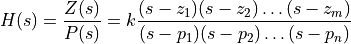
tf2zp(b, a)[source]¶

Convert transfer function filter parameters to zero-pole-gain form

Find the zeros, poles, and gains of this continuous-time system:

Warning

b and a must have the same length.

from spectrum import tf2zp
b = [2,3,0]
a = [1, 0.4, 1]
[z,p,k] = tf2zp(b,a)          % Obtain zero-pole-gain form
z =
    1.5
    0
p =
   -0.2000 + 0.9798i
    -0.2000 - 0.9798i
k =
   2

Parameters:

b – numerator
a – denominator
fill – If True, check that the length of a and b are the same. If not, create a copy of the shortest element and append zeros to it.

Returns:

z (zeros), p (poles), g (gain)

Convert transfer function f(x)=sum(b*x^n)/sum(a*x^n) to zero-pole-gain form f(x)=g*prod(1-z*x)/prod(1-p*x)

Todo

See if tf2ss followed by ss2zp gives better results. These are available from the control system toolbox. Note that the control systems toolbox doesn’t bother, but instead uses

See also

scipy.signal.tf2zpk, which gives the same results but uses a different algorithm (z^-1 instead of z).

tf2zpk(b, a)[source]¶

Return zero, pole, gain (z,p,k) representation from a numerator, denominator representation of a linear filter.

Convert zero-pole-gain filter parameters to transfer function form

Parameters:

b (ndarray) – numerator polynomial.
a (ndarray) – numerator and denominator polynomials.

Returns:

z : ndarray Zeros of the transfer function.
p : ndarray Poles of the transfer function.
k : float System gain.

If some values of b are too close to 0, they are removed. In that case, a BadCoefficients warning is emitted.

>>> import scipy.signal
>>> from spectrum.transfer import tf2zpk
>>> [b, a] = scipy.signal.butter(3.,.4)
>>> z, p ,k = tf2zpk(b,a)

See also

zpk2tf()

Note

wrapper of scipy function tf2zpk

zpk2ss(z, p, k)[source]¶

Zero-pole-gain representation to state-space representation

Parameters:

z,p (sequence) – Zeros and poles.
k (float) – System gain.

Returns:

A, B, C, D : ndarray State-space matrices.

Note

wrapper of scipy function zpk2ss

zpk2tf(z, p, k)[source]¶

Return polynomial transfer function representation from zeros and poles

Parameters:

z (ndarray) – Zeros of the transfer function.
p (ndarray) – Poles of the transfer function.
k (float) – System gain.

Returns:

b : ndarray Numerator polynomial. a : ndarray Numerator and denominator polynomials.

zpk2tf() forms transfer function polynomials from the zeros, poles, and gains of a system in factored form.

zpk2tf(z,p,k) finds a rational transfer function

$\frac{B(s)}{A(s)} = \frac{b_1 s^{n-1}+\dots b_{n-1}s+b_n}{a_1 s^{m-1}+\dots a_{m-1}s+a_m}$

given a system in factored transfer function form

$H(s) = \frac{Z(s)}{P(s)} = k \frac{(s-z_1)(s-z_2)\dots(s-z_m)}{(s-p_1)(s-p_2)\dots(s-p_n)}$

with p being the pole locations, and z the zero locations, with as many. The gains for each numerator transfer function are in vector k. The zeros and poles must be real or come in complex conjugate pairs. The polynomial denominator coefficients are returned in row vector a and the polynomial numerator coefficients are returned in matrix b, which has as many rows as there are columns of z.

Inf values can be used as place holders in z if some columns have fewer zeros than others.

Note

wrapper of scipy function zpk2tf

5.5.6. Waveforms ¶

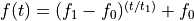
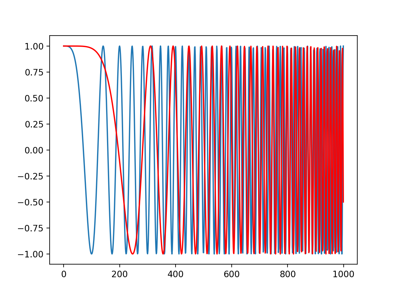
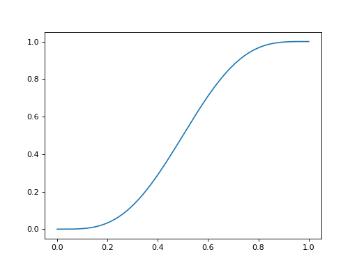
chirp(t, f0=0.0, t1=1.0, f1=100.0, form='linear', phase=0)[source]¶

Evaluate a chirp signal at time t.

A chirp signal is a frequency swept cosine wave.

$a = \pi (f_1 - f_0) / t_1$

$b = 2 \pi f_0$

$y = \cos\left( \pi\frac{f_1-f_0}{t_1} t^2 + 2\pi f_0 t + \rm{phase} \right)$

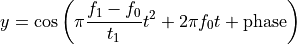
Parameters:

t (array) – times at which to evaluate the chirp signal
f0 (float) – frequency at time t=0 (Hz)
t1 (float) – time t1
f1 (float) – frequency at time t=t1 (Hz)
form (str) – shape of frequency sweep in [‘linear’, ‘quadratic’, ‘logarithmic’]
phase (float) – phase shift at t=0

The parameter form can be:

‘linear’ $f(t) = (f_1-f_0)(t/t_1) + f_0$

‘quadratic’ $f(t) = (f_1-f_0)(t/t_1)^2 + f_0$

‘logarithmic’ $f(t) = (f_1-f_0)^{(t/t_1)} + f_0$

Example:

from spectrum import chirp
from pylab import linspace, plot
t = linspace(0, 1, 1000)
y = chirp(t, form='linear')
plot(y)
y = chirp(t, form='quadratic')
plot(y, 'r')

(Source code, png, hires.png, pdf)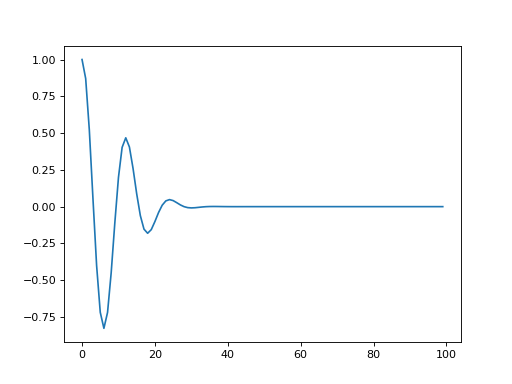

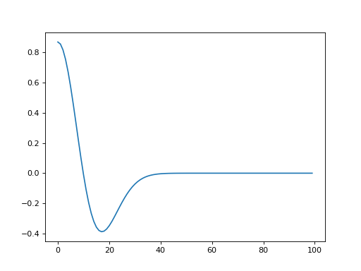
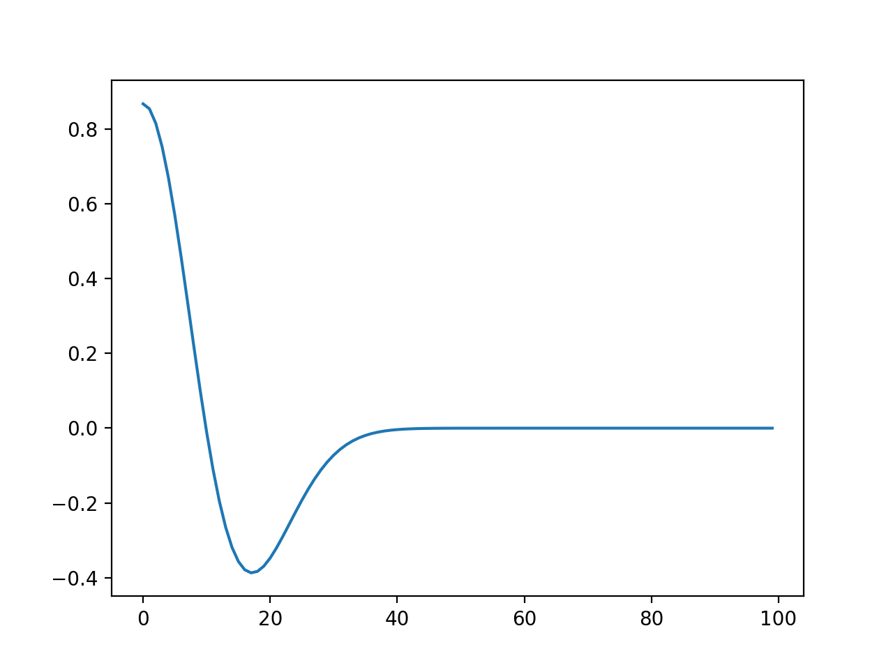
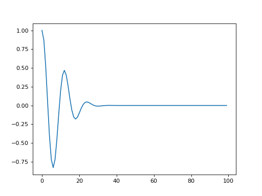
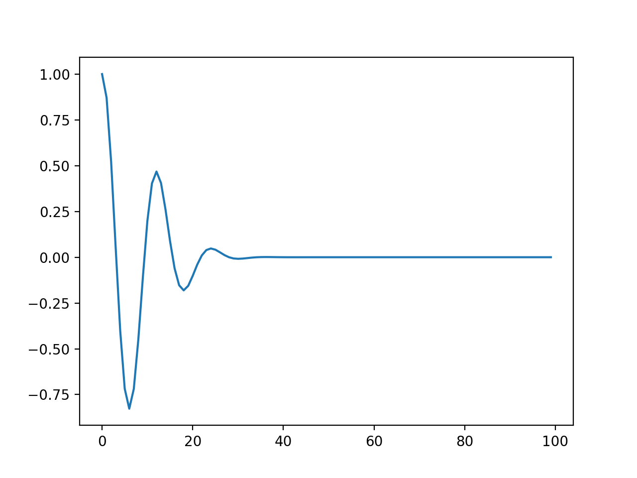
mexican(lb, ub, n)[source]¶

Generate the mexican hat wavelet

The Mexican wavelet is:

$w[x] = \cos{5x} \exp^{-x^2/2}$

Parameters:

lb – lower bound
ub – upper bound
n (int) – waveform data samples

Returns:

the waveform

from spectrum import mexican
from pylab import plot
plot(mexican(0, 10, 100))

(Source code, png, hires.png, pdf)

meyeraux(x)[source]¶

Compute the Meyer auxiliary function

The Meyer function is

$y = 35 x^4-84 x^5+70 x^6-20 x^7$

Parameters:: x (array)
Returns:: the waveform

from spectrum import meyeraux
from pylab import linspace, plot
t = linspace(0, 1, 1000)
plot(t, meyeraux(t))

(Source code, png, hires.png, pdf)

morlet(lb, ub, n)[source]¶

Generate the Morlet waveform

The Morlet waveform is defined as follows:

$w[x] = \cos{5x} \exp^{-x^2/2}$

Parameters:

lb – lower bound
ub – upper bound
n (int) – waveform data samples

from spectrum import morlet
from pylab import plot
plot(morlet(0,10,100))

(Source code, png, hires.png, pdf)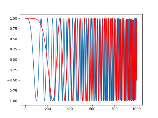

5.5.7. Linear prediction ¶

Linear prediction tools

References:: [Kay]

ac2poly(data)[source]¶

Convert autocorrelation sequence to prediction polynomial

Parameters:

data (array) – input data (list or numpy.array)

Returns:

AR parameters
noise variance

This is an alias to:

a, e, c = LEVINSON(data)

Example:

>>> from spectrum import ac2poly
>>> from numpy import array
>>> r = [5, -2, 1.01]
>>> ar, e = ac2poly(r)
>>> ar
array([ 1.  ,  0.38, -0.05])
>>> e
4.1895000000000007

ac2rc(data)[source]¶

Convert autocorrelation sequence to reflection coefficients

Parameters:: data – an autorrelation vector
Returns:: the reflection coefficient and data[0]

This is an alias to:

a, e, c = LEVINSON(data)
c, data[0]

is2rc(inv_sin)[source]¶

Convert inverse sine parameters to reflection coefficients.

Parameters:: inv_sin – inverse sine parameters
Returns:: reflection coefficients

Reference:: J.R. Deller, J.G. Proakis, J.H.L. Hansen, “Discrete-Time Processing of Speech Signals”, Prentice Hall, Section 7.4.5.

lar2rc(g)[source]¶

Convert log area ratios to reflection coefficients.

Parameters:: g – log area ratios
Returns:: the reflection coefficients

References:: [1] J. Makhoul, “Linear Prediction: A Tutorial Review,” Proc. IEEE, Vol.63, No.4, pp.561-580, Apr 1975.

lsf2poly(lsf)[source]¶

Convert line spectral frequencies to prediction filter coefficients

returns a vector a containing the prediction filter coefficients from a vector lsf of line spectral frequencies.

>>> from spectrum import lsf2poly
>>> lsf = [0.7842 ,   1.5605  ,  1.8776 ,   1.8984,    2.3593]
>>> a = lsf2poly(lsf)

# array([ 1.00000000e+00, 6.14837835e-01, 9.89884967e-01, # 9.31594056e-05, 3.13713832e-03, -8.12002261e-03 ])

See also

poly2lsf, rc2poly, ac2poly, rc2is

poly2ac(poly, efinal)[source]¶

Convert prediction filter polynomial to autocorrelation sequence

Parameters:

poly (array) – the AR parameters
efinal – an estimate of the final error

Returns:

the autocorrelation sequence in complex format.

>>> from numpy import array
>>> from spectrum import poly2ac
>>> poly = [ 1. ,  0.38 , -0.05]
>>> efinal = 4.1895
>>> poly2ac(poly, efinal)
array([ 5.00+0.j, -2.00+0.j,  1.01-0.j])

poly2lsf(a)[source]¶

Prediction polynomial to line spectral frequencies.

converts the prediction polynomial specified by A, into the corresponding line spectral frequencies, LSF. normalizes the prediction polynomial by A(1).

>>> from spectrum import poly2lsf
>>> a = [1.0000,  0.6149, 0.9899, 0.0000 ,0.0031, -0.0082]
>>> lsf = poly2lsf(a)
>>> lsf =  array([0.7842, 1.5605, 1.8776, 1.8984, 2.3593])

See also

lsf2poly, poly2rc, poly2qc, rc2is

poly2rc(a, efinal)[source]¶

Convert prediction filter polynomial to reflection coefficients

Parameters:

a – AR parameters
efinal

rc2ac(k, R0)[source]¶

Convert reflection coefficients to autocorrelation sequence.

Parameters:

k – reflection coefficients
R0 – zero-lag autocorrelation

Returns:

the autocorrelation sequence

rc2is(k)[source]¶

Convert reflection coefficients to inverse sine parameters.

Parameters:: k – reflection coefficients
Returns:: inverse sine parameters

See also

is2rc(), rc2poly(), rc2acC(), rc2lar().

Reference: J.R. Deller, J.G. Proakis, J.H.L. Hansen, “Discrete-Time: Processing of Speech Signals”, Prentice Hall, Section 7.4.5.

rc2lar(k)[source]¶

Convert reflection coefficients to log area ratios.

Parameters:: k – reflection coefficients
Returns:: inverse sine parameters

The log area ratio is defined by G = log((1+k)/(1-k)) , where the K parameter is the reflection coefficient.

See also

lar2rc(), rc2poly(), rc2ac(), rc2ic().

References:: [1] J. Makhoul, “Linear Prediction: A Tutorial Review,” Proc. IEEE, Vol.63, No.4, pp.561-580, Apr 1975.

rc2poly(kr, r0=None)[source]¶

convert reflection coefficients to prediction filter polynomial

Parameters:: k – reflection coefficients

5.5. Tools and classes ¶

5.5.1. Classes ¶

5.5.2. Correlation ¶

5.5.3. Tools ¶

5.5.4. datasets ¶

5.5.5. Linear Algebra Tools ¶

5.5.5.1. cholesky ¶

5.5.5.2. eigen ¶

5.5.5.3. levinson ¶

5.5.5.4. toeplitz ¶

5.5.5.5. linalg ¶

5.5.5.6. Transfer function ¶

5.5.6. Waveforms ¶

5.5.7. Linear prediction ¶

Table of Contents

Previous topic

Next topic

`CORRELATION`(x[, y, maxlags, norm])	Correlation function
`xcorr`(x[, y, maxlags, norm])	Cross-correlation using numpy.correlate

`db2mag`(xdb)	Convert decibels (dB) to magnitude
`db2pow`(xdb)	Convert decibels (dB) to power
`mag2db`(x)	Convert magnitude to decibels (dB)
`nextpow2`(x)	returns the smallest power of two that is greater than or equal to the absolute value of x.
`pow2db`(x)	returns the corresponding decibel (dB) value for a power value x.
`onesided_2_twosided`(data)	Convert a two-sided PSD to a one-sided PSD
`twosided_2_onesided`(data)	Convert a one-sided PSD to a twosided PSD
`centerdc_2_twosided`(data)	Convert a center-dc PSD to a twosided PSD
`twosided_2_centerdc`(data)	Convert a two-sided PSD to a center-dc PSD

`data_cosine`([N, A, sampling, freq])	Return a noisy cosine at a given frequency.
`marple_data`	64-complex data length from Marple reference [Marple]
`TimeSeries`(data[, sampling])	A simple Base Class for various data sets.

`csvd`(A)	SVD decomposition using numpy.linalg.svd
`corrmtx`(x_input, m[, method])	Correlation matrix
`pascal`(n)	Return Pascal matrix