5.1. Fourier Methods
5.1.1. Power Spectrum Density based on Fourier Spectrum
- default_NFFT = 4096
default number of samples used to compute FFT
Usage
You can compute a periodogram using speriodogram():
from spectrum import speriodogram, marple_data
from pylab import plot
p = speriodogram(marple_data)
plot(p)
However, the output is not always easy to manipulate or plot, therefore
it is advised to use the class Periodogram instead:
from spectrum import Periodogram, marple_data
p = Periodogram(marple_data)
p.plot()
This class will take care of the plotting and internal state of the computation. For instance, if you can change the output easily:
p.plot(sides='twosided')
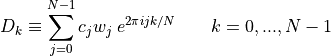
- DaniellPeriodogram(data, P, NFFT=None, detrend='mean', sampling=1.0, scale_by_freq=True, window='hamming')[source]
Return Daniell’s periodogram.
To reduce fast fluctuations of the spectrum one idea proposed by daniell is to average each value with points in its neighboorhood. It’s like a low filter.
![\hat{P}_D[f_i]= \frac{1}{2P+1} \sum_{n=i-P}^{i+P} \tilde{P}_{xx}[f_n]](_images/math/433b0367d9e13f14aaa0c10aebcd69b0b12ee11b.png)
where P is the number of points to average.
Daniell’s periodogram is the convolution of the spectrum with a low filter:
Example:
>>> DaniellPeriodogram(data, 8)
if N/P is not integer, the final values of the original PSD are not used.
using DaniellPeriodogram(data, 0) should give the original PSD.
- class Periodogram(data, sampling=1.0, window='hann', NFFT=None, scale_by_freq=False, detrend=None)[source]
The Periodogram class provides an interface to periodogram PSDs
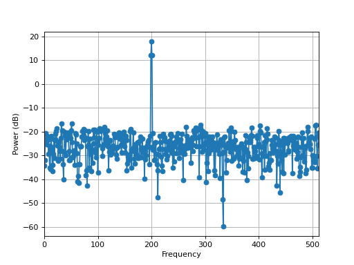
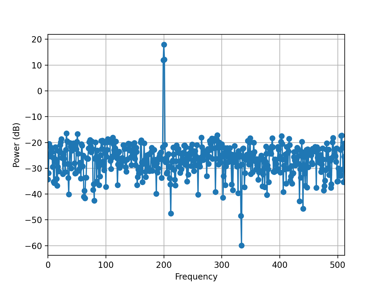
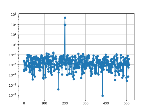
from spectrum import Periodogram, data_cosine
data = data_cosine(N=1024, A=0.1, sampling=1024, freq=200)
p = Periodogram(data, sampling=1024)
p.plot(marker='o')
(
Source code,png,hires.png,pdf)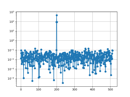
Periodogram Constructor
- WelchPeriodogram(data, NFFT=None, sampling=1.0, **kargs)[source]
Simple periodogram wrapper of numpy.psd function.
- Parameters:
- Technical documentation:
When we calculate the periodogram of a set of data we get an estimation of the spectral density. In fact as we use a Fourier transform and a truncated segments the spectrum is the convolution of the data with a rectangular window which Fourier transform is
![W(s)= \frac{1}{N^2} \left[ \frac{\sin(\pi s)}{\sin(\pi s/N)} \right]^2](_images/math/202252a9e70abd803229b3d656855119bb9d18c0.png)
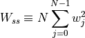
Thus oscillations and sidelobes appears around the main frequency. One aim of t he tapering is to reduced this effects. We multiply data by a window whose sidelobes are much smaller than the main lobe. Classical window is hanning window. But other windows are available. However we must take into account this energy and divide the spectrum by energy of taper used. Thus periodogram becomes :
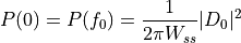
![P(f_k)=\frac{1}{2\pi W_{ss}} \left[\arrowvert{D_k}\arrowvert^2+\arrowvert{D_{N-k}}\arrowvert^2\right] \qquad k=0,1,..., \left( \frac{1}{2}-1 \right)](_images/math/cb39fa72d520c905248ba5255339f4ae474f2ccc.png)
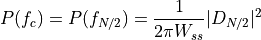
with
from spectrum import WelchPeriodogram, marple_data
psd = WelchPeriodogram(marple_data, 256)
(
Source code,png,hires.png,pdf)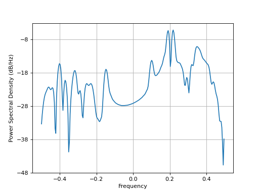
- class pdaniell(data, P, sampling=1.0, window='hann', NFFT=None, scale_by_freq=True, detrend=None)[source]
The pdaniell class provides an interface to DaniellPeriodogram
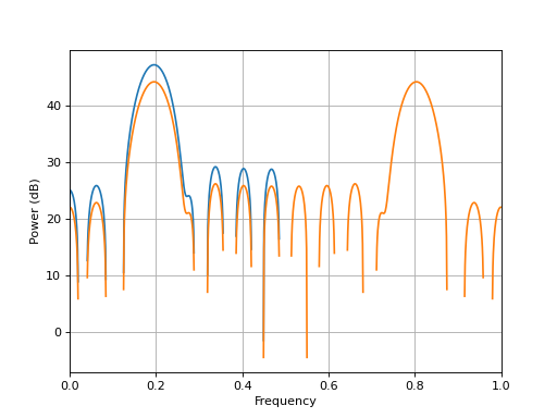
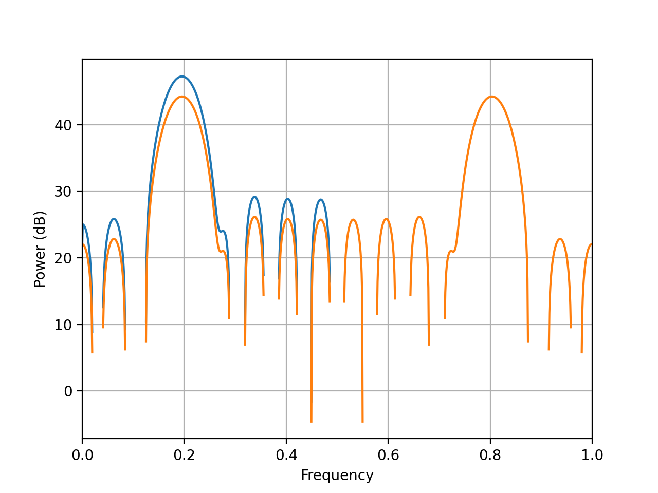
from spectrum import data_cosine, pdaniell
data = data_cosine(N=4096, sampling=4096)
p = pdaniell(data, 8, NFFT=4096)
p.plot()
pdaniell Constructor
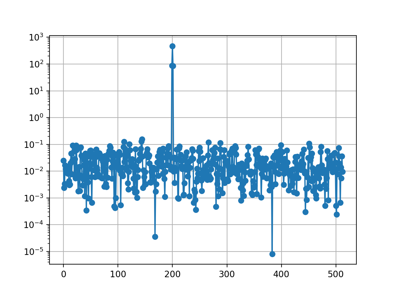
- speriodogram(x, NFFT=None, detrend=True, sampling=1.0, scale_by_freq=True, window='hamming', axis=0)[source]
Simple periodogram, but matrices accepted.
- Parameters:
- Returns:
2-sided PSD if complex data, 1-sided if real.
if a matrix is provided (using numpy.matrix), then a periodogram is computed for each row. The returned matrix has the same shape as the input matrix.
The mean of the input data is also removed from the data before computing the psd.
from pylab import grid, semilogy
from spectrum import data_cosine, speriodogram
data = data_cosine(N=1024, A=0.1, sampling=1024, freq=200)
semilogy(speriodogram(data, detrend=False, sampling=1024), marker='o')
grid(True)
(
Source code,png,hires.png,pdf)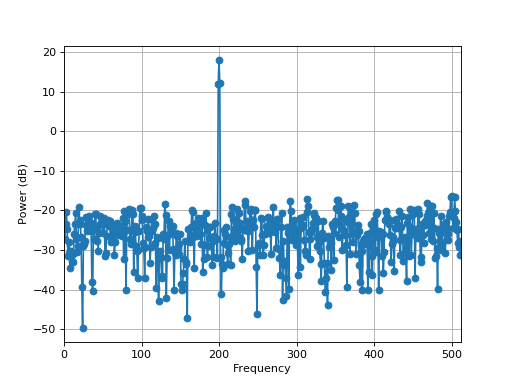
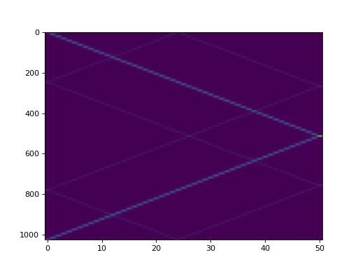
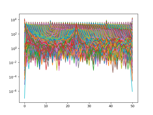
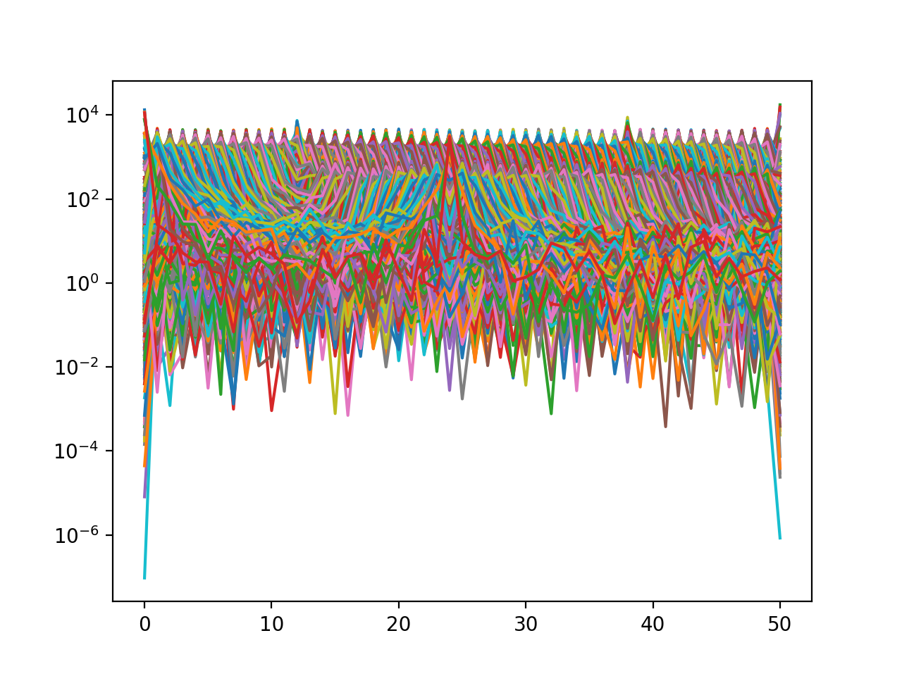
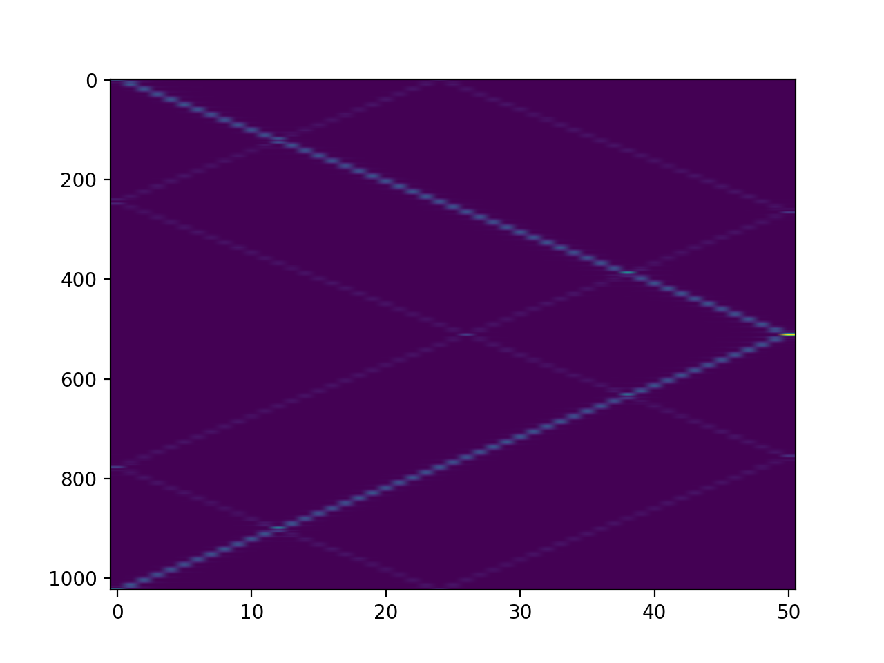
import numpy
from spectrum import speriodogram, data_cosine
from pylab import figure, semilogy, figure ,imshow
# create N data sets and make the frequency dependent on the time
N = 100
m = numpy.concatenate([data_cosine(N=1024, A=0.1, sampling=1024, freq=x)
    for x in range(1, N)]);
m.resize(N, 1024)
res = speriodogram(m)
figure(1)
semilogy(res)
figure(2)
imshow(res.transpose(), aspect='auto')

Todo
a proper spectrogram class/function that takes care of normalisation
Correlogram PSD estimates
- CORRELOGRAMPSD(X, Y=None, lag=-1, window='hamming', norm='unbiased', NFFT=4096, window_params={}, correlation_method='xcorr')[source]
PSD estimate using correlogram method.
- Parameters:
X (array) – complex or real data samples X(1) to X(N)
Y (array) – complex data samples Y(1) to Y(N). If provided, computes the cross PSD, otherwise the PSD is returned
lag (int) – highest lag index to compute. Must be less than N
norm (str) – one of the valid normalisation of
xcorr()(biased, unbiased, coeff, None)NFFT (int) – total length of the final data sets (padded with zero if needed; default is 4096)
correlation_method (str) – either xcorr or CORRELATION. CORRELATION should be removed in the future.
- Returns:
Array of real (cross) power spectral density estimate values. This is a two sided array with negative values following the positive ones whatever is the input data (real or complex).
Description:
The exact power spectral density is the Fourier transform of the autocorrelation sequence:
![P_{xx}(f) = T \sum_{m=-\infty}^{\infty} r_{xx}[m] exp^{-j2\pi fmT}](_images/math/0cdea2e00e08d54cc5172335a5cff5a295622e3f.png)
The correlogram method of PSD estimation substitutes a finite sequence of autocorrelation estimates
 in place of
  .
This estimation can be computed with
.
This estimation can be computed with xcorr()orCORRELATION()by chosing a proprer lag L. The estimated PSD is then![\hat{P}_{xx}(f) = T \sum_{m=-L}^{L} \hat{r}_{xx}[m] exp^{-j2\pi fmT}](_images/math/6ff2418ebfe4f016bf6654135affde77e71b27c8.png)
The lag index must be less than the number of data samples N. Ideally, it should be around L/10 [Marple] so as to avoid greater statistical variance associated with higher lags.
To reduce the leakage of the implicit rectangular window and therefore to reduce the bias in the estimate, a tapering window is normally used and lead to the so-called Blackman and Tukey correlogram:
![\hat{P}_{BT}(f) = T \sum_{m=-L}^{L} w[m] \hat{r}_{xx}[m] exp^{-j2\pi fmT}](_images/math/e2932a940e29aee6e3e2cd17e8aaebec72d8c006.png)
The correlogram for the cross power spectral estimate is
which is computed if
Yis not provide. In such case, so we compute the correlation only once.
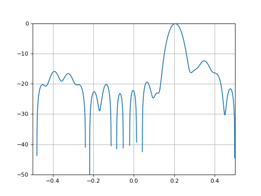
from spectrum import CORRELOGRAMPSD, marple_data
from spectrum.tools import cshift
from pylab import log10, axis, grid, plot,linspace

psd = CORRELOGRAMPSD(marple_data, marple_data, lag=15)
f = linspace(-0.5, 0.5, len(psd))
psd = cshift(psd, len(psd)/2)
plot(f, 10*log10(psd/max(psd)))
axis([-0.5,0.5,-50,0])
grid(True)
(
Source code,png,hires.png,pdf)
See also
create_window(),CORRELATION(),xcorr(),pcorrelogram.
- class pcorrelogram(data, sampling=1.0, lag=-1, window='hamming', NFFT=None, scale_by_freq=True, detrend=None)[source]
The Correlogram class provides an interface to
CORRELOGRAMPSD().It returns an object that inherits from
FourierSpectrumand therefore ease the manipulation of PSDs.from spectrum import pcorrelogram, data_cosine p = pcorrelogram(data_cosine(N=1024), lag=15) p.plot() p.plot(sides='twosided')
(
Source code,png,hires.png,pdf)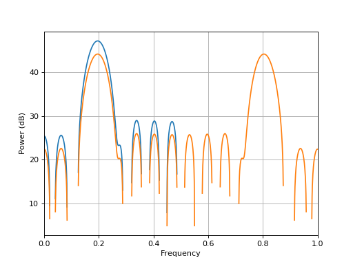
Correlogram Constructor
- Parameters:
5.1.2. Tapering Windows
- class Window(N, name=None, norm=True, **kargs)[source]
Window tapering object
This class provides utilities to manipulate tapering windows. Plotting functions allows to visualise the time and frequency response. It is also possible to retrieve relevant quantities such as the equivalent noise band width.
The following examples illustrates the usage. First, we create the window by providing a name and a size:
from spectrum import Window
w = Window(64, 'hamming')
The window has been computed and the data is stored in:
w.data
This object contains plotting methods so that you can see the time or frequency response.
from spectrum.window import Window
w = Window(64, 'hamming')
w.plot_frequencies()
(
Source code,png,hires.png,pdf)
Some windows may accept optional arguments. For instance,
window_blackman()accepts an optional argument called as well as
 Window. Indeed, we use the factorycreate_window(), which manage all the optional arguments. So you can write:w = Window(64, 'blackman', alpha=1)
See also
Constructor:
Create a tapering window object
- Parameters:
N – the window length
name – the type of window, e.g., ‘Hann’
norm – normalise the window in frequency domain (for plotting)
kargs – any of
create_window()valid optional arguments.
Attributes:
data: time series data
frequencies: getter to the frequency series
response: getter to the PSD
enbw: getter to the Equivalent noise band width.
- property N
Getter for the window length
- compute_response(**kargs)[source]
Compute the window data frequency response
- Parameters:
norm – True by default. normalised the frequency data.
NFFT (int) – total length of the final data sets( 2048 by default. if less than data length, then NFFT is set to the data length*2).
The response is stored in
response.Note
Units are dB (20 log10) since we plot the frequency response)
- property data
Getter for the window values (in time)
- property frequencies
Getter for the frequency array
- property mean_square
returns :math:` rac{w^2}{N}`
- property name
Getter for the window name
- property norm
Getter of the normalisation flag (True by default)
- plot_frequencies(mindB=None, maxdB=None, norm=True)[source]
Plot the window in the frequency domain
- Parameters:
mindB – change the default lower y bound
maxdB – change the default upper lower bound
norm (bool) – if True, normalise the frequency response.
from spectrum.window import Window
w = Window(64, name='hamming')
w.plot_frequencies()
(
Source code,png,hires.png,pdf)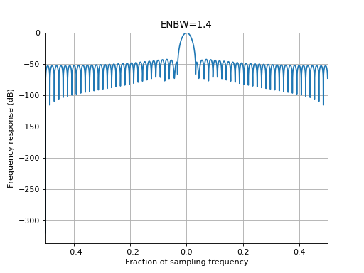
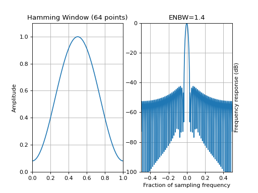
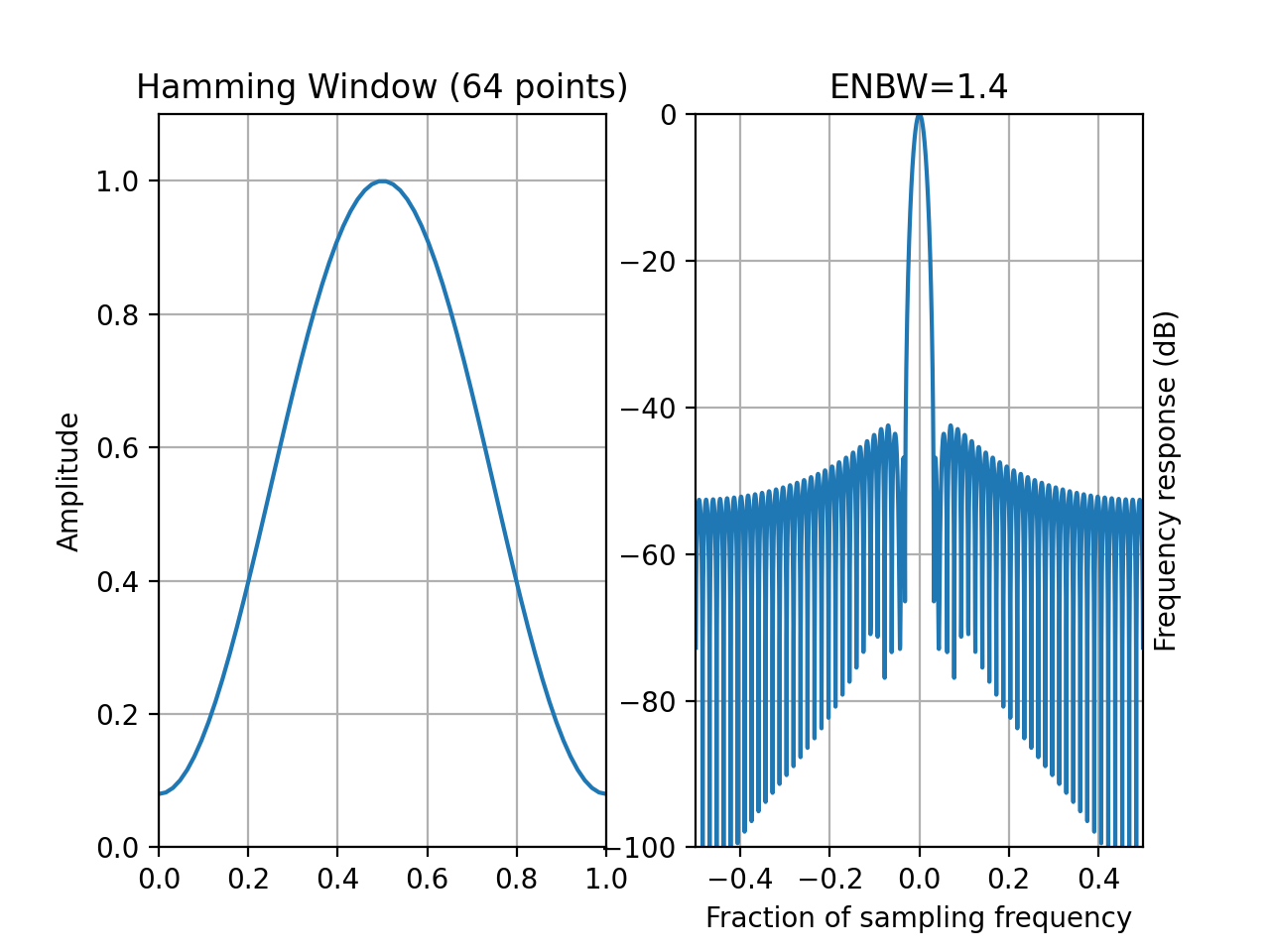
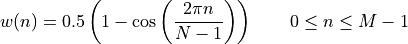
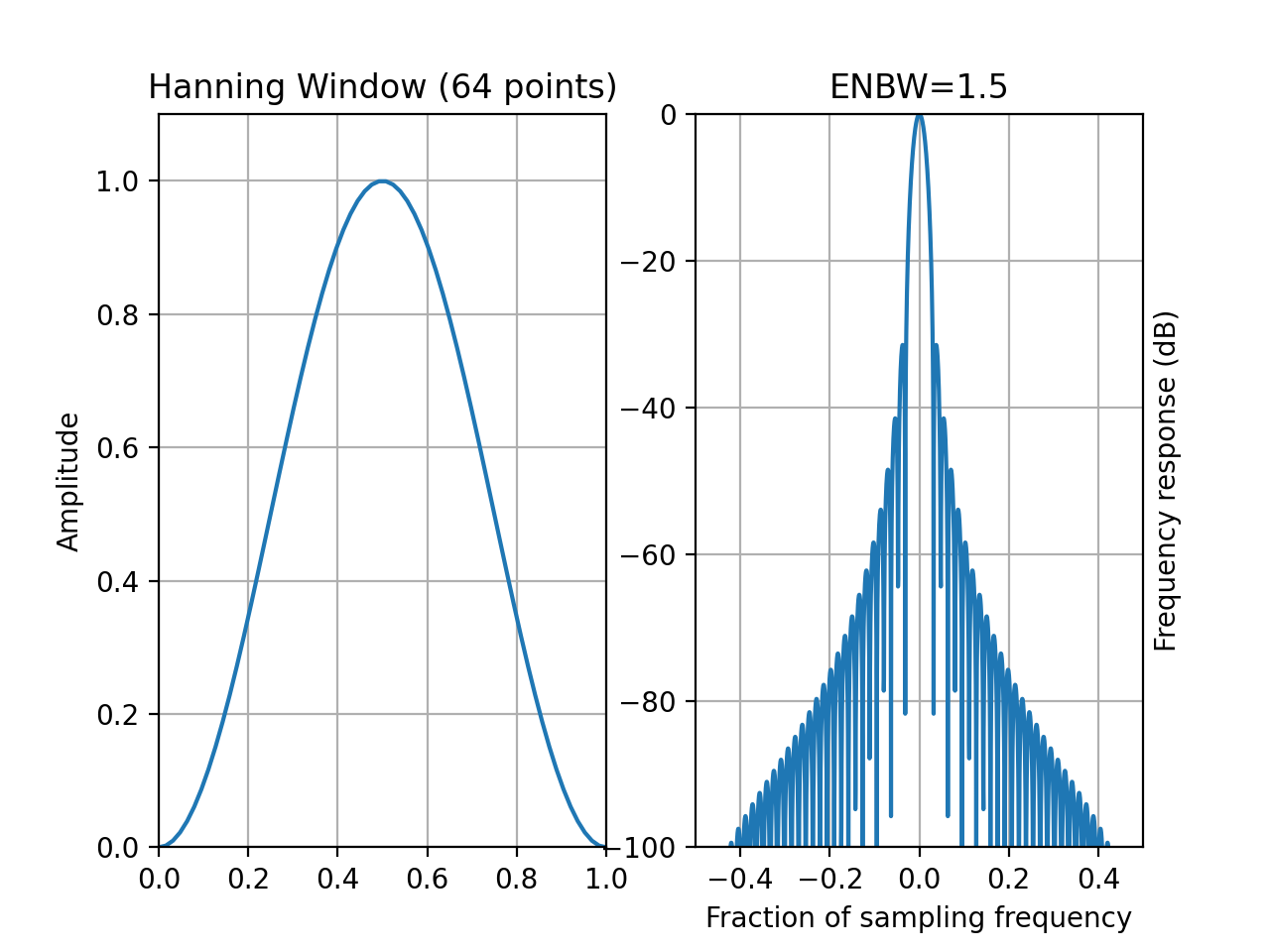
- plot_time_freq(mindB=-100, maxdB=None, norm=True, yaxis_label_position='right')[source]
Plotting method to plot both time and frequency domain results.
See
plot_frequencies()for the optional arguments.from spectrum.window import Window w = Window(64, name='hamming') w.plot_time_freq()
(
Source code,png,hires.png,pdf)
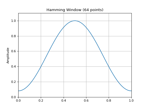
- plot_window()[source]
Plot the window in the time domain
from spectrum.window import Window
w = Window(64, name='hamming')
w.plot_window()
(
Source code,png,hires.png,pdf)
- property response
Getter for the frequency response. See
compute_response()
- create_window(N, name=None, **kargs)[source]
Returns the N-point window given a valid name
- Parameters:
N (int) – window size
name (str) – window name (default is rectangular). Valid names are stored in
window_names().kargs –
optional arguments are:
beta: argument of the
window_kaiser()function (default is 8.6)attenuation: argument of the
window_chebwin()function (default is 50dB)- alpha: argument of the
window_gaussian()function (default is 2.5)window_blackman()function (default is 0.16)window_poisson()function (default is 2)window_cauchy()function (default is 3)
mode: argument
window_flattop()function (default is symmetric, can be periodic)r: argument of the
window_tukey()function (default is 0.5).
The following windows have been simply wrapped from existing librairies like NumPy:
Rectangular:
window_rectangle(),Bartlett or Triangular: see
window_bartlett(),Hanning or Hann: see
window_hann(),Hamming: see
window_hamming(),Kaiser: see
window_kaiser(),chebwin: see
window_chebwin().
The following windows have been implemented from scratch:
Blackman: See
window_blackman()Bartlett-Hann : see
window_bartlett_hann()cosine or sine: see
window_cosine()gaussian: see
window_gaussian()Bohman: see
window_bohman()Lanczos or sinc: see
window_lanczos()Blackman Harris: see
window_blackman_harris()Blackman Nuttall: see
window_blackman_nuttall()Nuttall: see
window_nuttall()Tukey: see
window_tukey()Parzen: see
window_parzen()Flattop: see
window_flattop()Riesz: see
window_riesz()Riemann: see
window_riemann()Poisson: see
window_poisson()Poisson-Hanning: see
window_poisson_hanning()
Todo
on request taylor, potter, Bessel, expo, rife-vincent, Kaiser-Bessel derived (KBD)
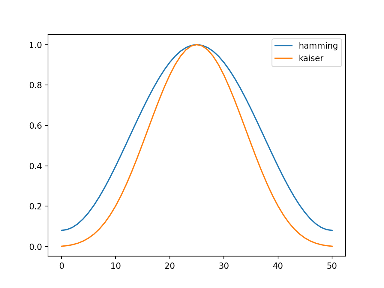
from pylab import plot, legend
from spectrum import create_window

data = create_window(51, 'hamming')
plot(data, label='hamming')
data = create_window(51, 'kaiser')
plot(data, label='kaiser')
legend()
(
Source code,png,hires.png,pdf)
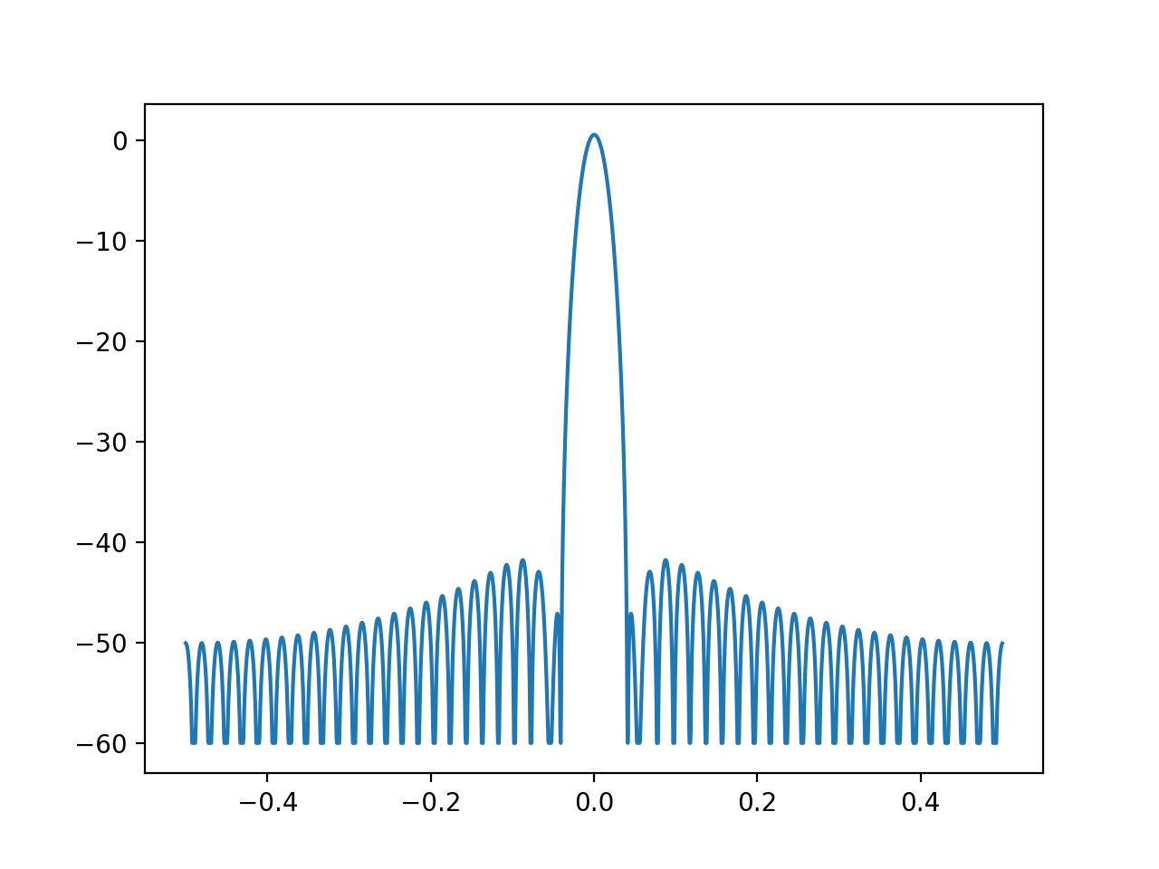
from pylab import plot, log10, linspace, fft, clip
from spectrum import create_window, fftshift

A = fft(create_window(51, 'hamming'), 2048) / 25.5
mag = abs(fftshift(A))
freq = linspace(-0.5,0.5,len(A))
response = 20 * log10(mag)
mindB = -60
response = clip(response,mindB,100)
plot(freq, response)
(
Source code,png,hires.png,pdf)
See also
window_visu(),Window(),spectrum.dpss
- enbw(data)[source]
Computes the equivalent noise bandwidth
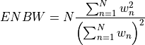
>>> from spectrum import create_window, enbw
>>> w = create_window(64, 'rectangular')
>>> enbw(w)
1.0
The following table contains the ENBW values for some of the implemented windows in this module (with N=16384). They have been double checked against litterature (Source: [Harris], [Marple]).
If not present, it means that it has not been checked.
name
ENBW
litterature
rectangular
triangle
1.3334
1.33
Hann
1.5001
1.5
Hamming
1.3629
1.36
blackman
1.7268
1.73
kaiser
1.7
blackmanharris,4
2.004
riesz
1.2000
1.2
riemann
1.32
1.3
parzen
1.917
1.92
tukey 0.25
1.102
1.1
bohman
1.7858
1.79
poisson 2
1.3130
1.3
hanningpoisson 0.5
1.609
1.61
cauchy
1.489
1.48
lanczos
1.3
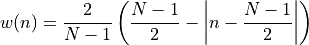
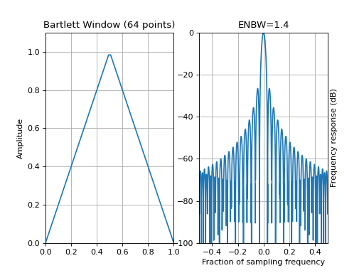
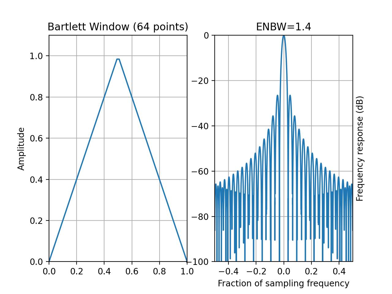
- window_bartlett(N)[source]
Bartlett window (wrapping of numpy.bartlett) also known as Fejer
- Parameters:
N (int) – window length
The Bartlett window is defined as
from spectrum import window_visu
window_visu(64, 'bartlett')
(
Source code,png,hires.png,pdf)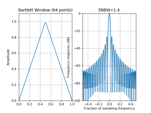
See also
numpy.bartlett,
create_window(),Window.
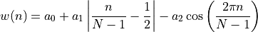
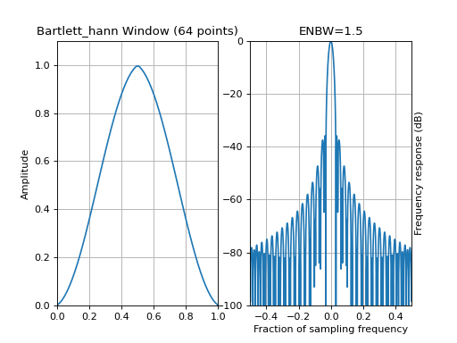
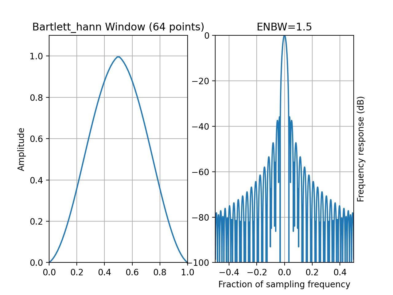
- window_bartlett_hann(N)[source]
Bartlett-Hann window
- Parameters:
N – window length
with
 ,
,  and
and 
from spectrum import window_visu
window_visu(64, 'bartlett_hann')
(
Source code,png,hires.png,pdf)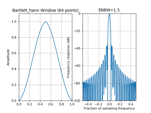
See also
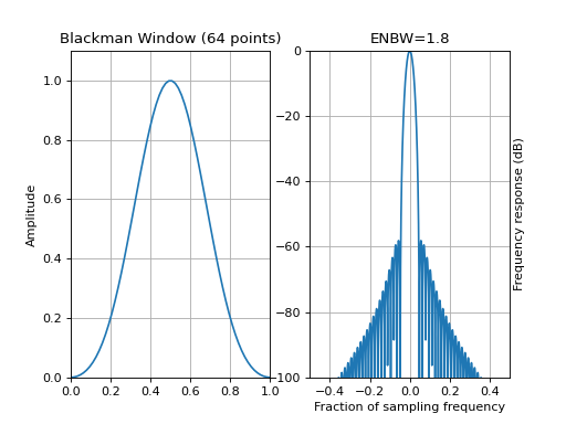
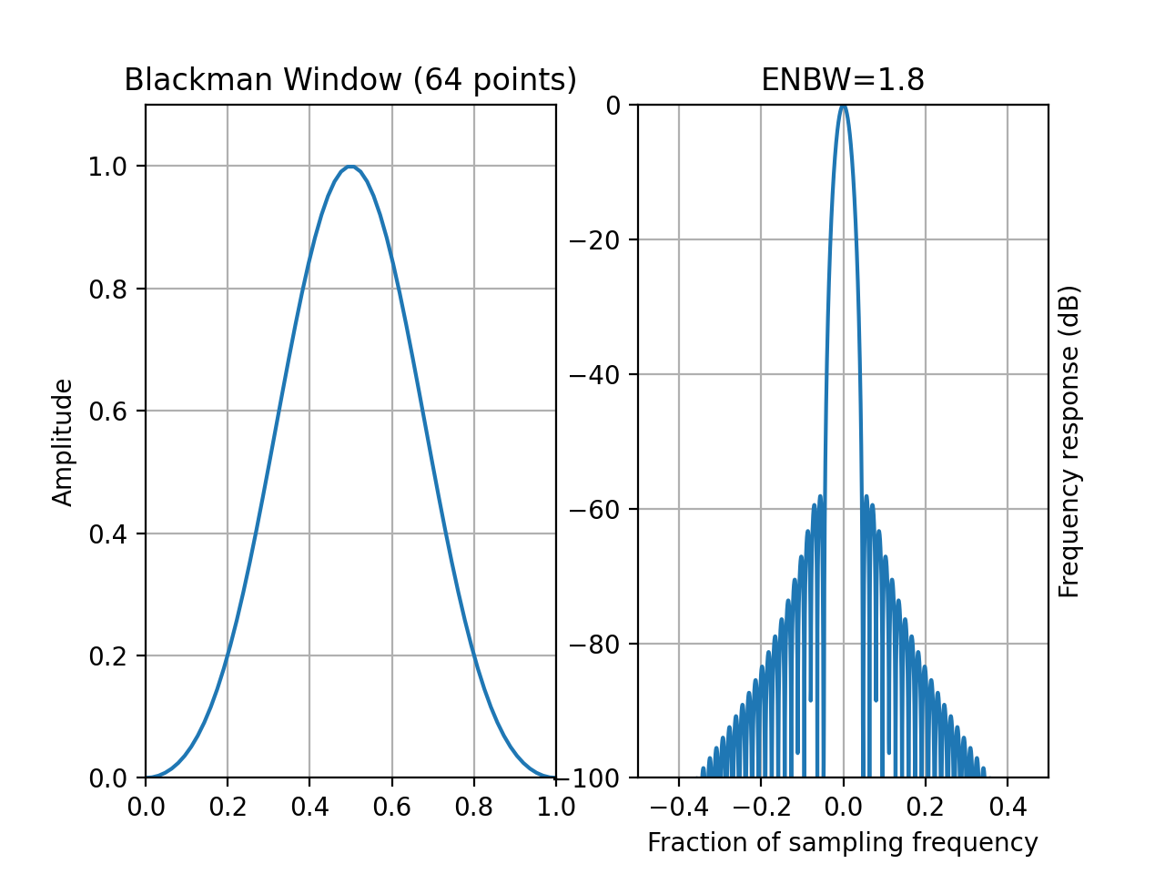
- window_blackman(N, alpha=0.16)[source]
Blackman window
- Parameters:
N – window length
with

When
 , this is the unqualified Blackman window with
 and
and  .
.from spectrum import window_visu window_visu(64, 'blackman')
(
Source code,png,hires.png,pdf)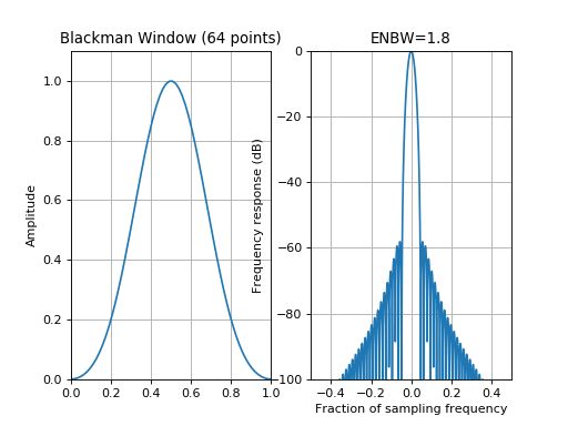
Note
Although Numpy implements a blackman window for
,
this implementation is valid for any .See also
numpy.blackman,
create_window(),Window
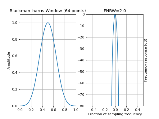
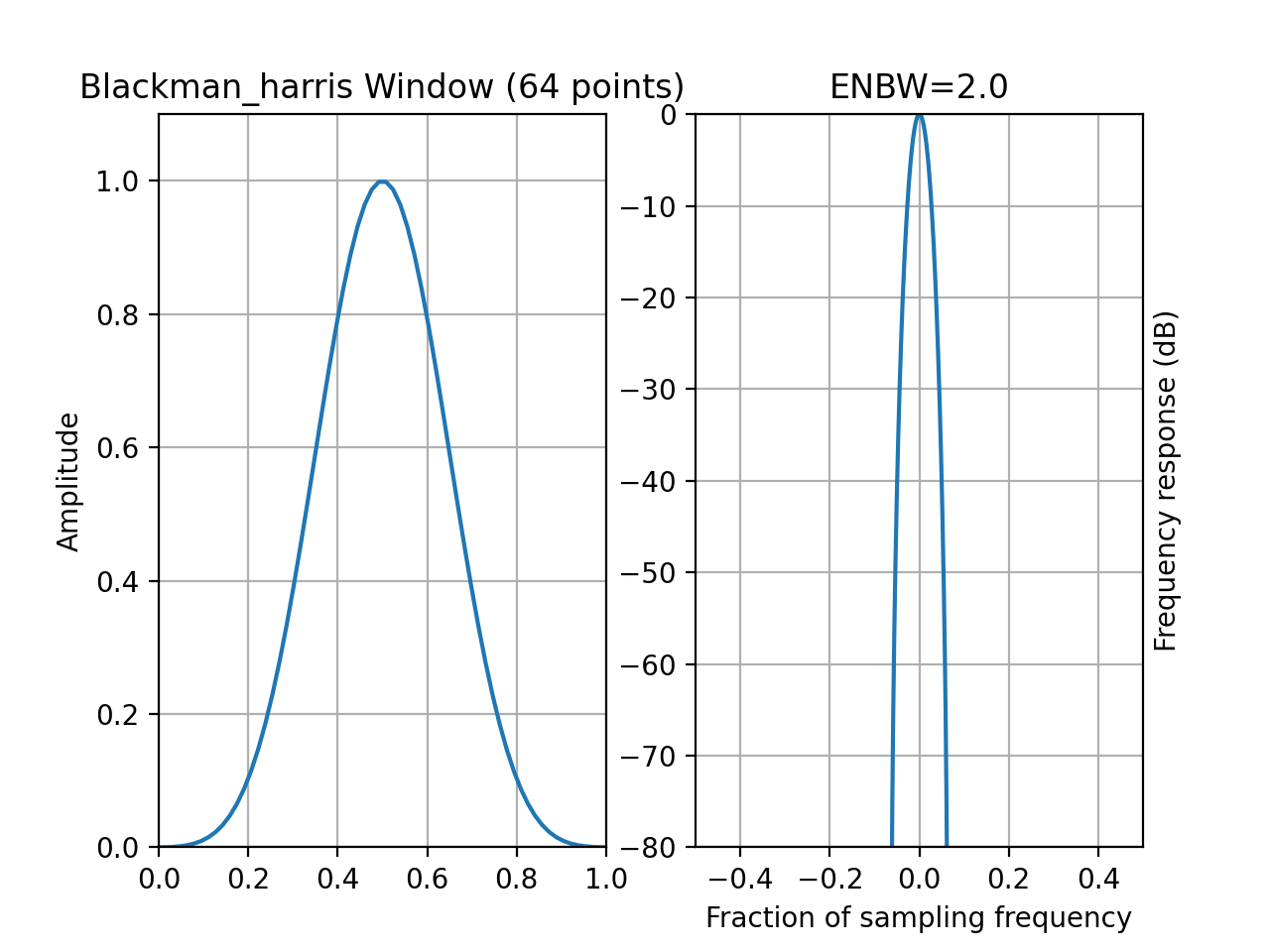
- window_blackman_harris(N)[source]
Blackman Harris window
- Parameters:
N – window length

coeff
value

0.35875

0.48829

0.14128

0.01168
from spectrum import window_visu
window_visu(64, 'blackman_harris', mindB=-80)
(
Source code,png,hires.png,pdf)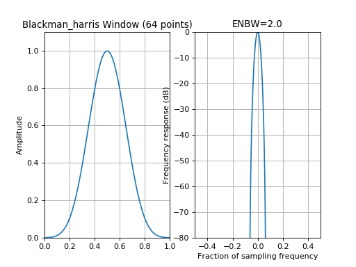
See also
See also
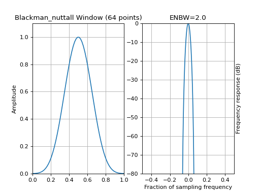
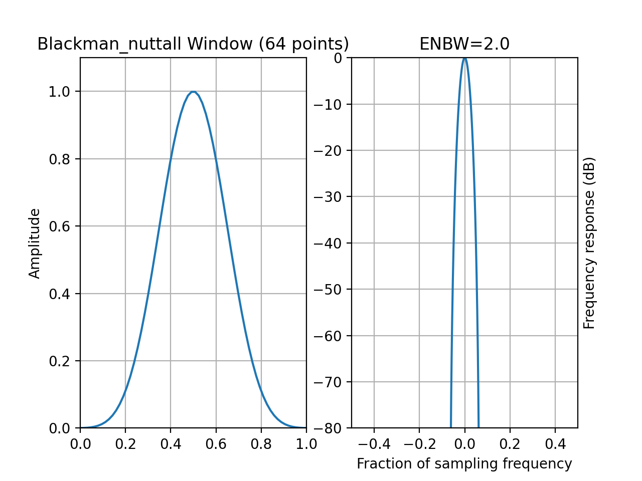
- window_blackman_nuttall(N)[source]
Blackman Nuttall window
returns a minimum, 4-term Blackman-Harris window. The window is minimum in the sense that its maximum sidelobes are minimized. The coefficients for this window differ from the Blackman-Harris window coefficients and produce slightly lower sidelobes.
- Parameters:
N – window length
with
 ,
,  ,
,  and
and 
from spectrum import window_visu
window_visu(64, 'blackman_nuttall', mindB=-80)
(
Source code,png,hires.png,pdf)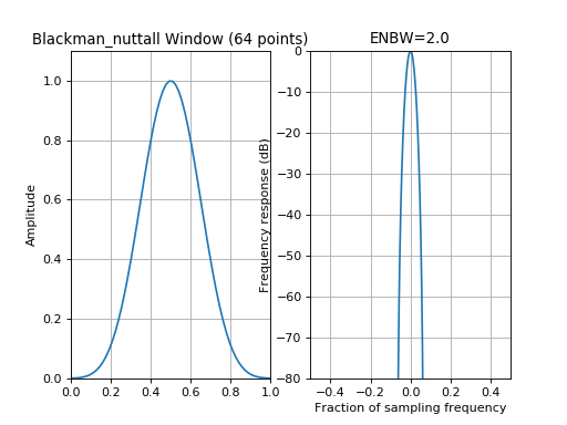
See also
See also
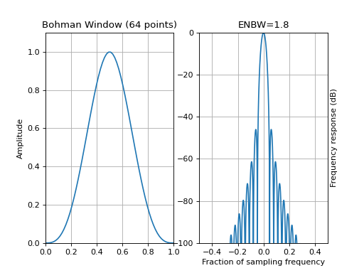
- window_bohman(N)[source]
Bohman tapering window
- Parameters:
N – window length
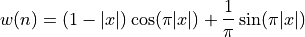
where x is a length N vector of linearly spaced values between -1 and 1.
from spectrum import window_visu
window_visu(64, 'bohman')
(
Source code,png,hires.png,pdf)
See also
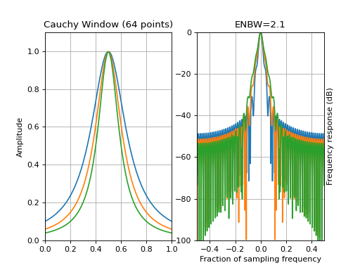
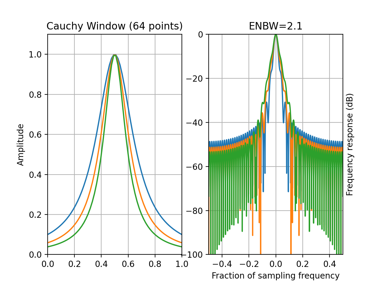
- window_cauchy(N, alpha=3)[source]
Cauchy tapering window
from spectrum import window_visu
window_visu(64, 'cauchy', alpha=3)
window_visu(64, 'cauchy', alpha=4)
window_visu(64, 'cauchy', alpha=5)
(
Source code,png,hires.png,pdf)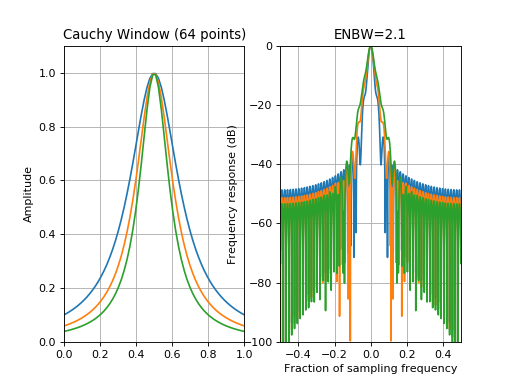
See also
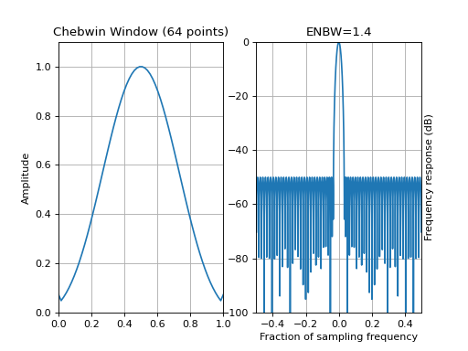
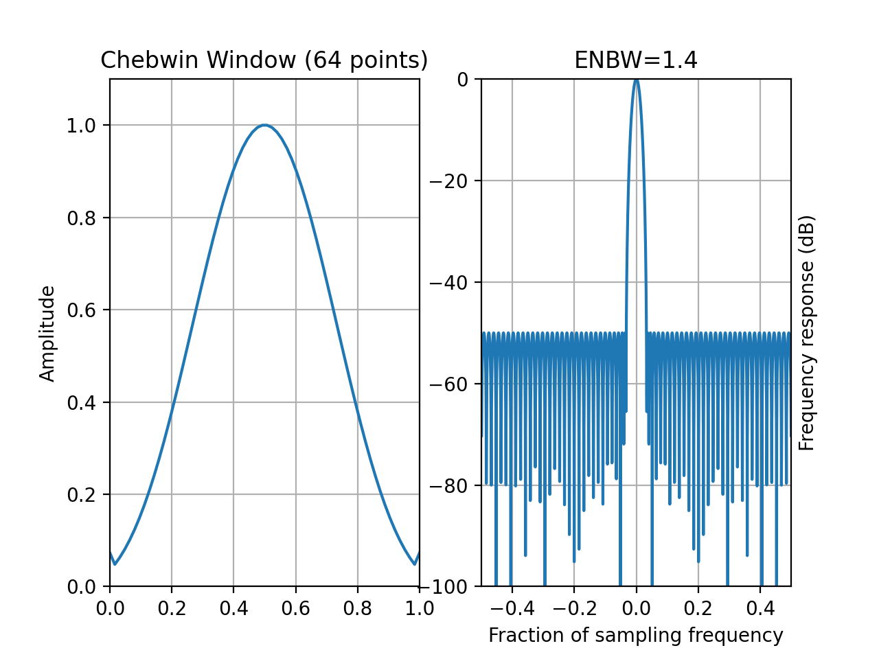
- window_chebwin(N, attenuation=50)[source]
Cheb window
- Parameters:
N – window length
from spectrum import window_visu
window_visu(64, 'chebwin', attenuation=50)
(
Source code,png,hires.png,pdf)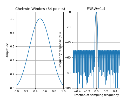
See also
scipy.signal.chebwin,
create_window(),Window
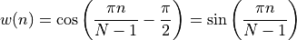
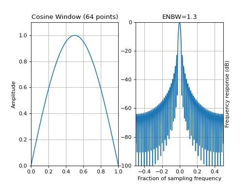
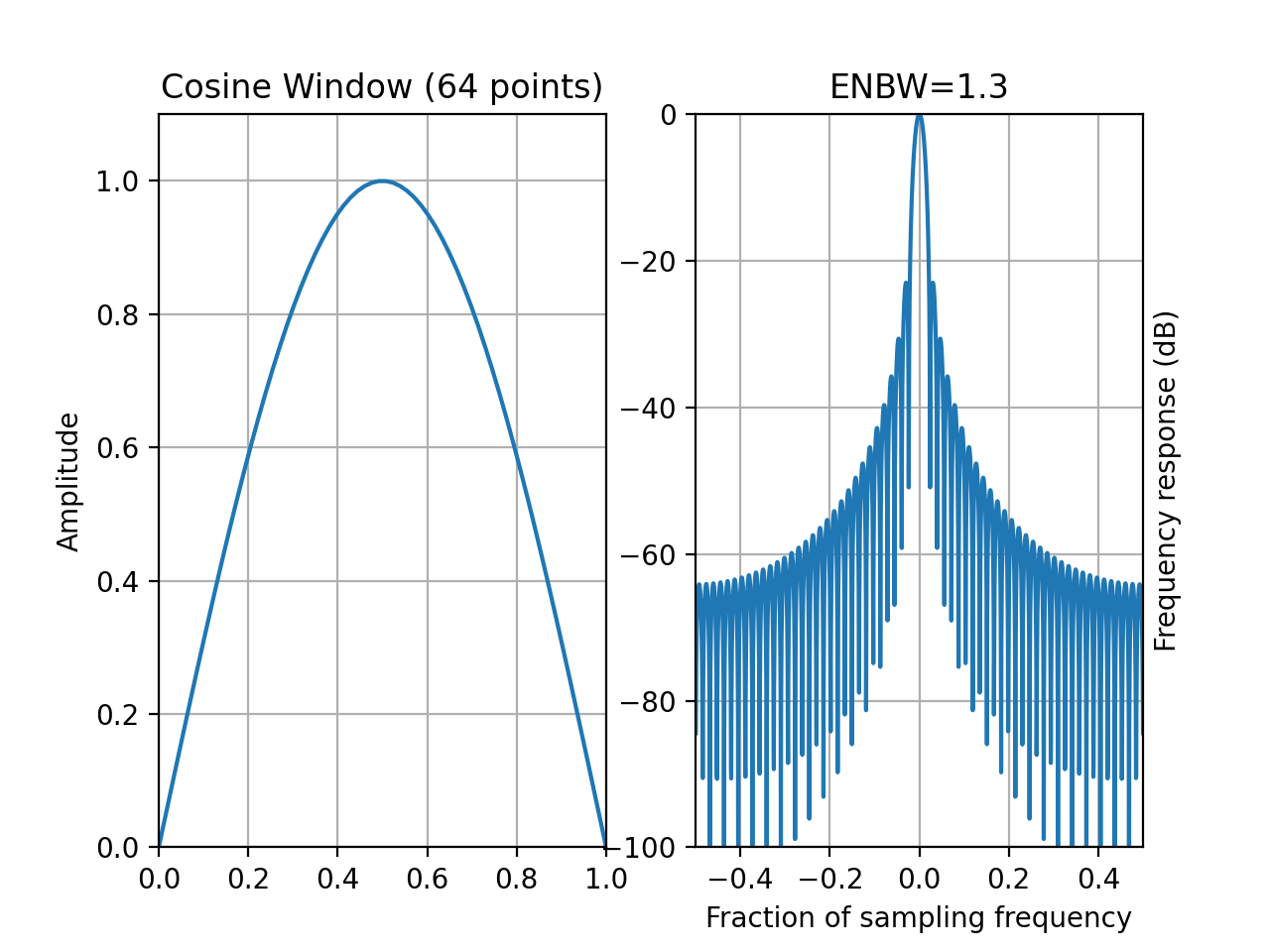
- window_cosine(N)[source]
Cosine tapering window also known as sine window.
- Parameters:
N – window length
from spectrum import window_visu
window_visu(64, 'cosine')
(
Source code,png,hires.png,pdf)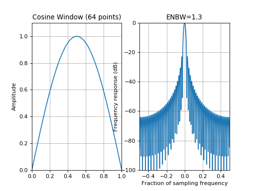
See also
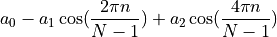
- window_flattop(N, mode='symmetric', precision=None)[source]
Flat-top tapering window
Returns symmetric or periodic flat top window.
- Parameters:
N – window length
mode – way the data are normalised. If mode is symmetric, then divide n by N-1. IF mode is periodic, divide by N, to be consistent with octave code.
When using windows for filter design, the symmetric mode should be used (default). When using windows for spectral analysis, the periodic mode should be used. The mathematical form of the flat-top window in the symmetric case is:

coeff
value
a0
0.21557895
a1
0.41663158
a2
0.277263158
a3
0.083578947
a4
0.006947368
from spectrum import window_visu
window_visu(64, 'bohman')
(
Source code,png,hires.png,pdf)
See also
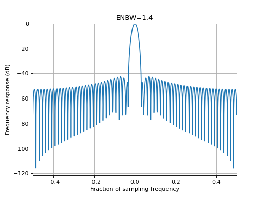
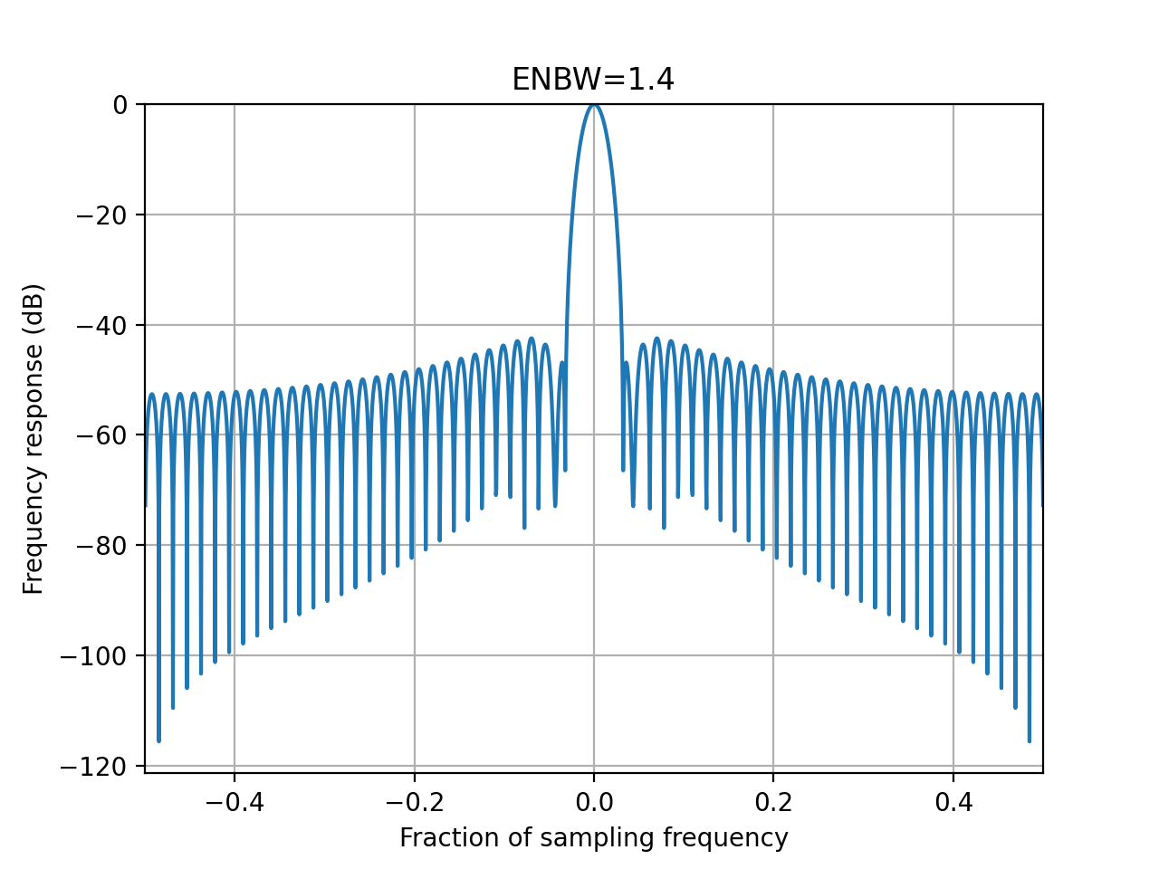
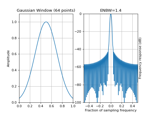
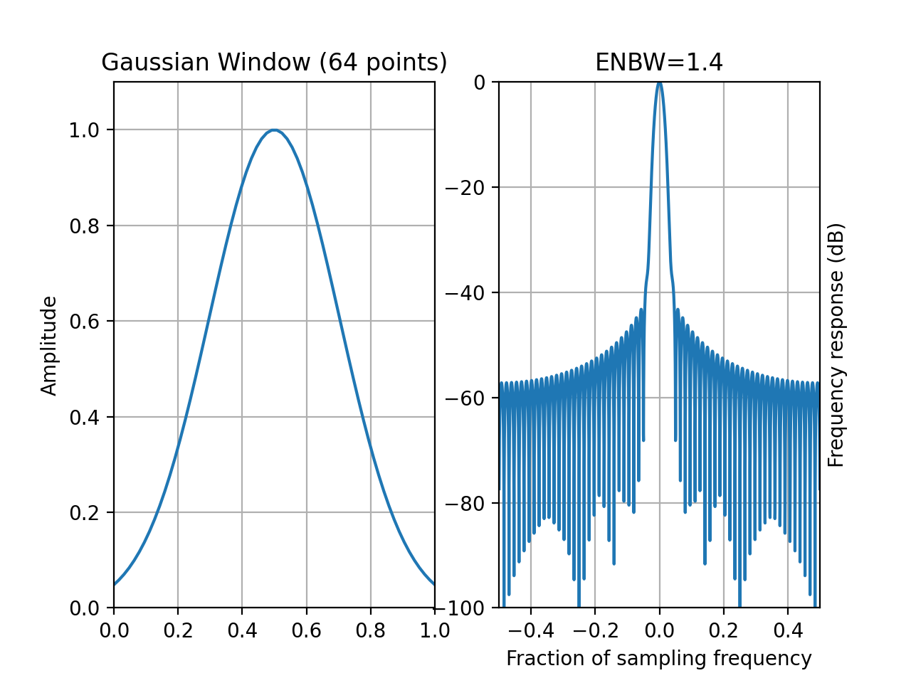
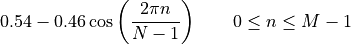
- window_gaussian(N, alpha=2.5)[source]
Gaussian window
- Parameters:
N – window length
with
 .
.Note
N-1 is used to be in agreement with octave convention. The ENBW of 1.4 is also in agreement with [Harris]
from spectrum import window_visu
window_visu(64, 'gaussian', alpha=2.5)
(
Source code,png,hires.png,pdf)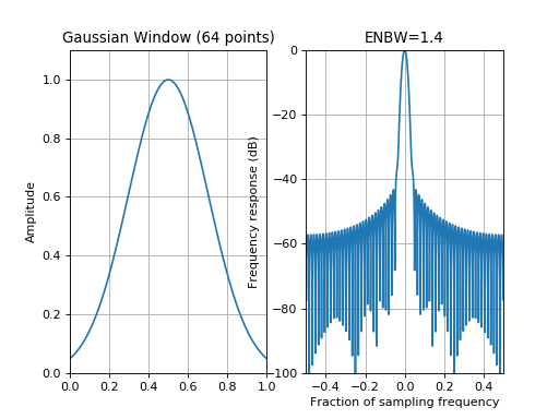
See also
scipy.signal.gaussian,
create_window()
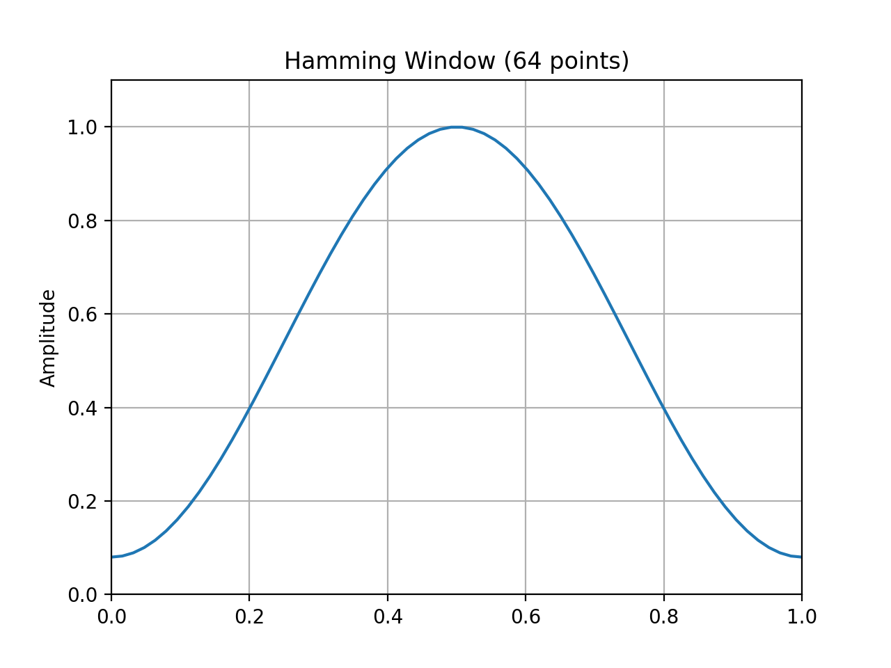
- window_hamming(N)[source]
Hamming window
- Parameters:
N – window length
The Hamming window is defined as
from spectrum import window_visu
window_visu(64, 'hamming')
(
Source code,png,hires.png,pdf)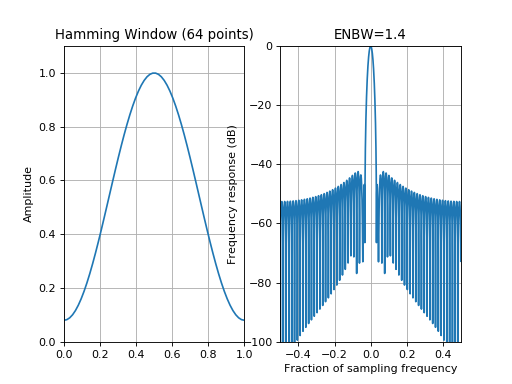
See also
numpy.hamming,
create_window(),Window.
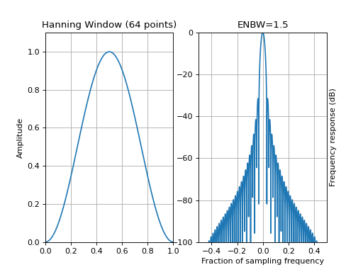
- window_hann(N)[source]
Hann window (or Hanning). (wrapping of numpy.bartlett)
- Parameters:
N (int) – window length
The Hanning window is also known as the Cosine Bell. Usually, it is called Hann window, to avoid confusion with the Hamming window.
from spectrum import window_visu
window_visu(64, 'hanning')
(
Source code,png,hires.png,pdf)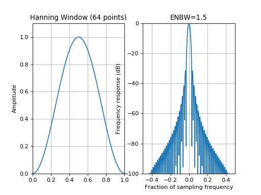
See also
numpy.hanning,
create_window(),Window.
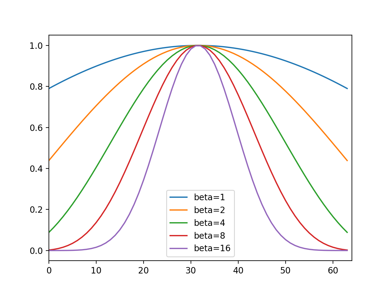
- window_kaiser(N, beta=8.6, method='numpy')[source]
Kaiser window
- Parameters:
N – window length
beta – kaiser parameter (default is 8.6)
To obtain a Kaiser window that designs an FIR filter with sidelobe attenuation of
dB, use the following  where
where
 .
.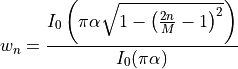
where
 is the zeroth order Modified Bessel function of the first kind.
- is a real number that determines the shape of the
window. It determines the trade-off between main-lobe width and side
lobe level.
the length of the sequence is N=M+1.
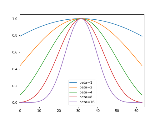
The Kaiser window can approximate many other windows by varying the
parameter:beta
Window shape
0
Rectangular
5
Similar to a Hamming
6
Similar to a Hanning
8.6
Similar to a Blackman
from pylab import plot, legend, xlim
from spectrum import window_kaiser
N = 64
for beta in [1,2,4,8,16]:
    plot(window_kaiser(N, beta), label='beta='+str(beta))
xlim(0,N)
legend()
(
Source code,png,hires.png,pdf)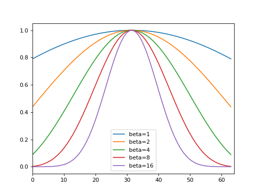
from spectrum import window_visu
window_visu(64, 'kaiser', beta=8.)
(
Source code,png,hires.png,pdf)
See also
numpy.kaiser,
spectrum.window.create_window()
- window_lanczos(N)[source]
Lanczos window also known as sinc window.
- Parameters:
N – window length
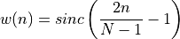
from spectrum import window_visu
window_visu(64, 'lanczos')
(
Source code,png,hires.png,pdf)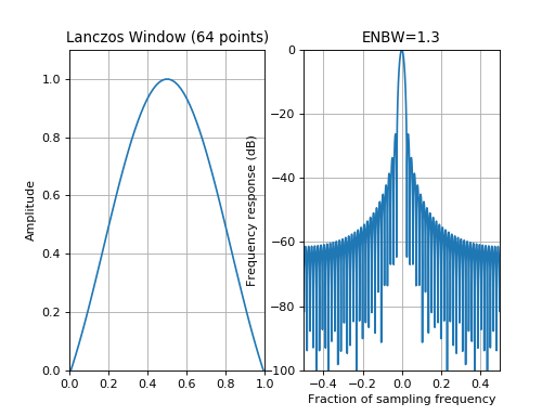
See also
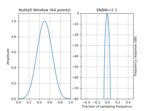
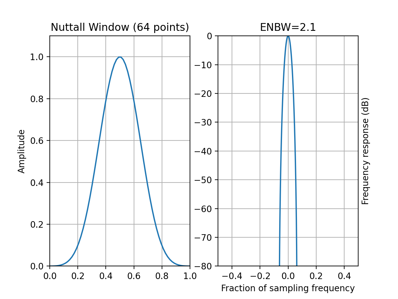
- window_nuttall(N)[source]
Nuttall tapering window
- Parameters:
N – window length
with
 ,
,  ,
,  and
and 
from spectrum import window_visu
window_visu(64, 'nuttall', mindB=-80)
(
Source code,png,hires.png,pdf)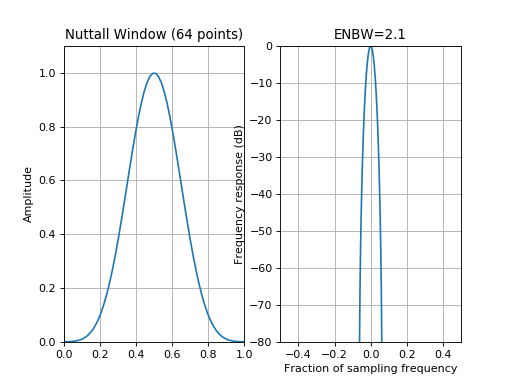
See also
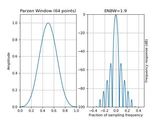
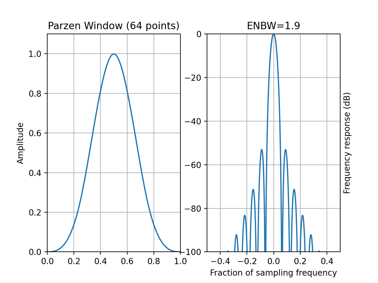
- window_parzen(N)[source]
Parsen tapering window (also known as de la Valle-Poussin)
- Parameters:
N – window length
Parzen windows are piecewise cubic approximations of Gaussian windows. Parzen window sidelobes fall off as
 .
.if
 :
: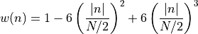
if

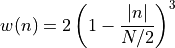
from spectrum import window_visu
window_visu(64, 'parzen')
(
Source code,png,hires.png,pdf)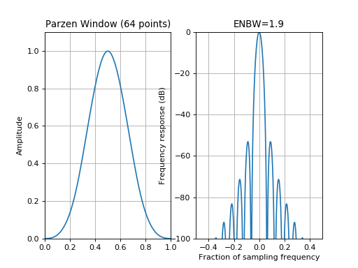
See also
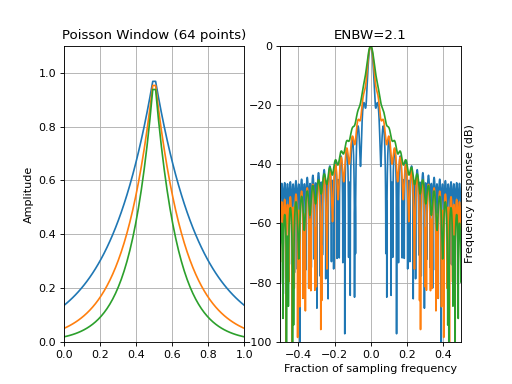
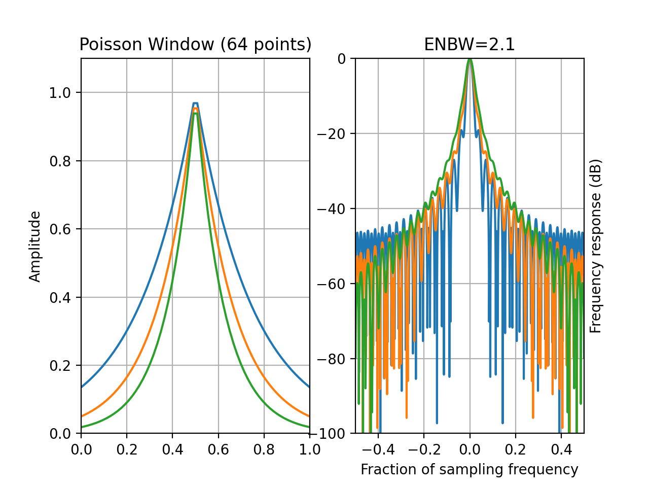
- window_poisson(N, alpha=2)[source]
Poisson tapering window
- Parameters:
N (int) – window length
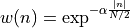
with
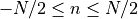 .
.from spectrum import window_visu window_visu(64, 'poisson') window_visu(64, 'poisson', alpha=3) window_visu(64, 'poisson', alpha=4)
(
Source code,png,hires.png,pdf)
See also
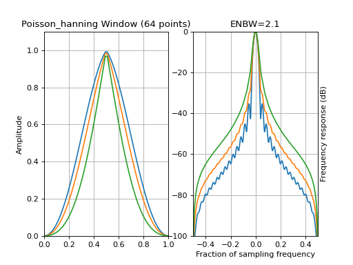
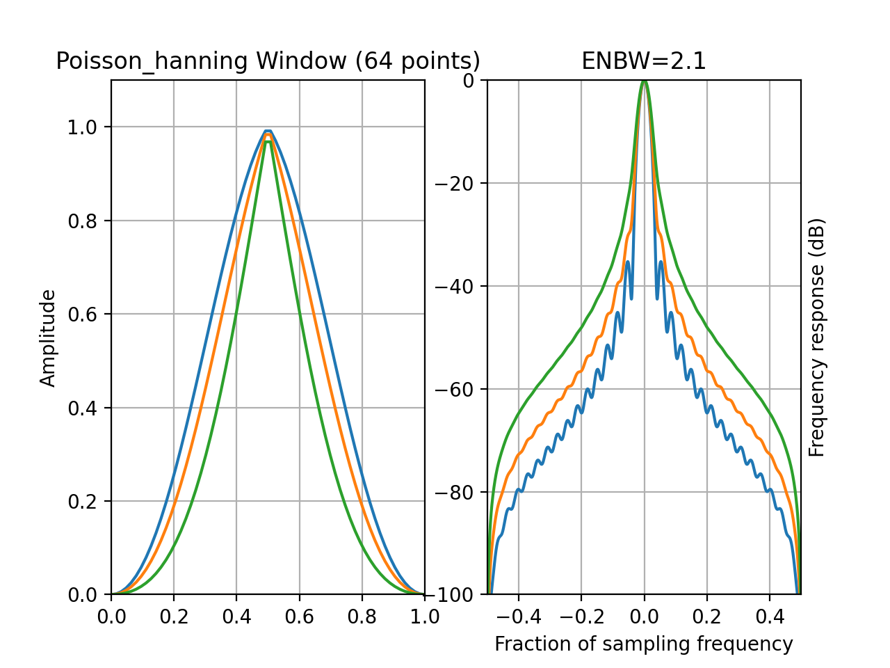
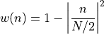
- window_poisson_hanning(N, alpha=2)[source]
Hann-Poisson tapering window
This window is constructed as the product of the Hanning and Poisson windows. The parameter alpha is the Poisson parameter.
from spectrum import window_visu
window_visu(64, 'poisson_hanning', alpha=0.5)
window_visu(64, 'poisson_hanning', alpha=1)
window_visu(64, 'poisson_hanning')
(
Source code,png,hires.png,pdf)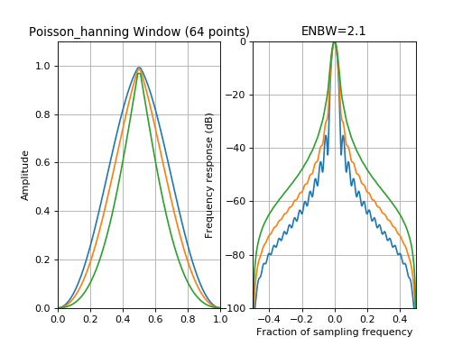
See also
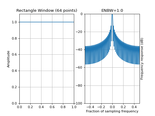
- window_rectangle(N)[source]
Kaiser window
- Parameters:
N – window length
from spectrum import window_visu
window_visu(64, 'rectangle')
(
Source code,png,hires.png,pdf)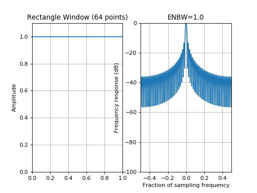
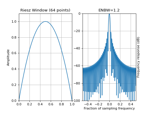
- window_riemann(N)[source]
Riemann tapering window
- Parameters:
N (int) – window length
with
.from spectrum import window_visu window_visu(64, 'riesz')
(
Source code,png,hires.png,pdf)
See also
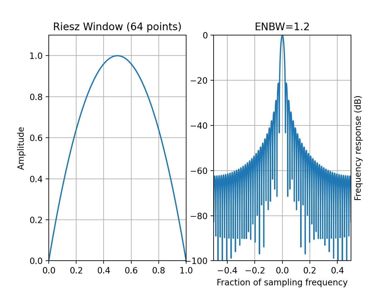
- window_riesz(N)[source]
Riesz tapering window
- Parameters:
N – window length
with
.from spectrum import window_visu window_visu(64, 'riesz')
(
Source code,png,hires.png,pdf)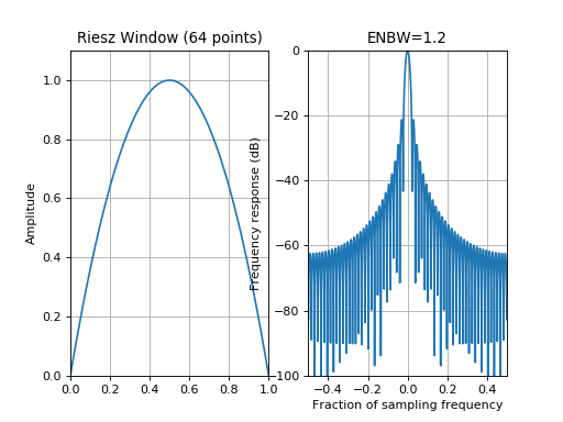
See also
- window_taylor(N, nbar=4, sll=-30)[source]
Taylor tapering window
Taylor windows allows you to make tradeoffs between the mainlobe width and sidelobe level (sll).
Implemented as described by Carrara, Goodman, and Majewski in ‘Spotlight Synthetic Aperture Radar: Signal Processing Algorithms’ Pages 512-513
The default values gives equal height sidelobes (nbar) and maximum sidelobe level (sll).
Warning
not implemented
See also
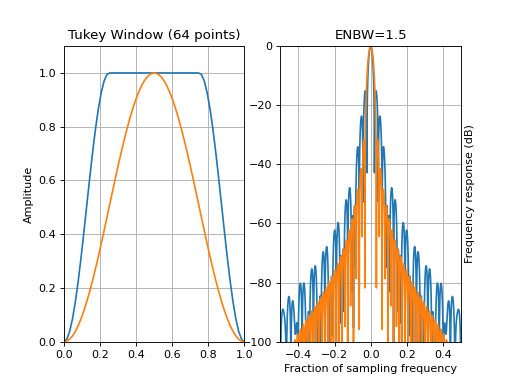
- window_tukey(N, r=0.5)[source]
Tukey tapering window (or cosine-tapered window)
- Parameters:
N – window length
r – defines the ratio between the constant section and the cosine section. It has to be between 0 and 1.
The function returns a Hanning window for r=0 and a full box for r=1.
from spectrum import window_visu
window_visu(64, 'tukey')
window_visu(64, 'tukey', r=1)
(
Source code,png,hires.png,pdf)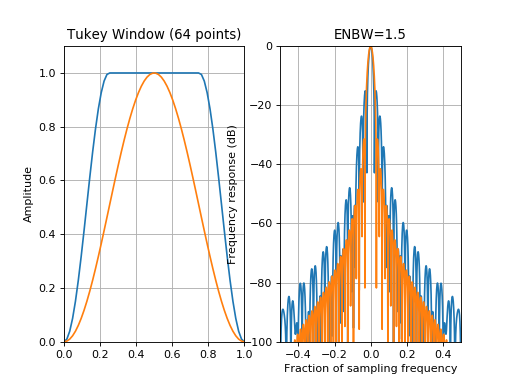


See also
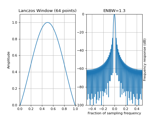
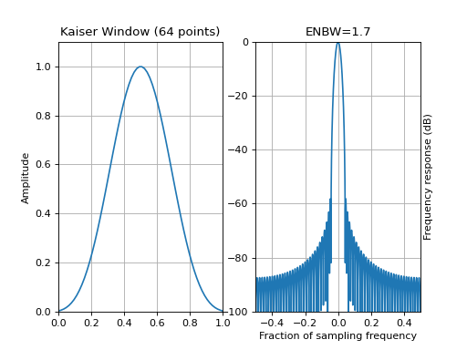
- window_visu(N=51, name='hamming', **kargs)[source]
A Window visualisation tool
- Parameters:
N – length of the window
name – name of the window
NFFT – padding used by the FFT
mindB – the minimum frequency power in dB
maxdB – the maximum frequency power in dB
kargs – optional arguments passed to
create_window()
This function plot the window shape and its equivalent in the Fourier domain.
from spectrum import window_visu
window_visu(64, 'kaiser', beta=8.)
(
Source code,png,hires.png,pdf)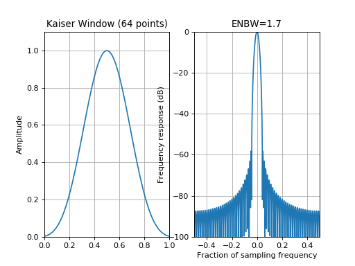